Modeling Transient Compressible Flow

Objective

This example models transient, compressible airflow through a nozzle, mimicking jet engine or rocket propulsion systems. It starts with a steady-state solution to establish an accurate initial flow field. A time-varying outlet pressure, defined by a sinusoidal expression, simulates pulsating flow.

The simulation uses a density-based solver to capture shock waves and automatic mesh adaptation to refine the grid in high-gradient regions, like shocks. This ensures numerical stability and accuracy in both steady and transient phases. The approach demonstrates steady-to-transient coupling, dynamic boundary conditions, and adaptive meshing for high-speed, time-dependent flows.

Problem Description

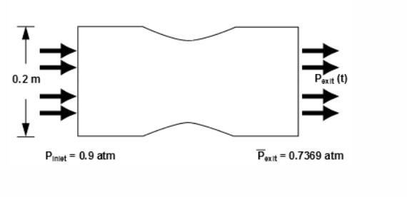
The nozzle has an inlet height of 0.2 meters and a smooth, sinusoidal contour that reduces the cross-sectional flow area by 20% at the throat, accelerating air to high Mach numbers. This design mimics jet engine nozzles, where flow compression drives thrust. Due to geometric and flow symmetry along the center plane, only half the domain is modeled, reducing computational cost while maintaining accurate flow field results, including shock formation and pressure dynamics.

Import modules

Note

Importing the following classes offer streamlined access to key solver settings, eliminating the need to manually browse through the full settings structure.

import os
import platform

import ansys.fluent.core as pyfluent
from ansys.fluent.core import examples
from ansys.fluent.core.solver import (
    BoundaryConditions,
    CellRegisters,
    Contour,
    Controls,
    General,
    Graphics,
    Initialization,
    Mesh,
    PressureInlet,
    PressureOutlet,
    ReportDefinitions,
    ReportFiles,
    ReportPlots,
    RunCalculation,
    Setup,
)
from ansys.fluent.visualization import GraphicsWindow, Monitor

Launch Fluent session in meshing mode

session = pyfluent.launch_fluent(mode="meshing")

meshing = session.workflow

Meshing workflow

filenames = {
    "Windows": "nozzle.dsco",
    "Other": "nozzle.dsco.pmdb",
}

geometry_filename = examples.download_file(
    filenames.get(platform.system(), filenames["Other"]),
    "pyfluent/transient_compressible_simulation",
    save_path=os.getcwd(),
)

meshing.InitializeWorkflow(WorkflowType="Watertight Geometry")
meshing.TaskObject["Import Geometry"].Arguments = {"FileName": geometry_filename}
meshing.TaskObject["Import Geometry"].Execute()

meshing.TaskObject["Add Local Sizing"].Execute()

Generate surface mesh

surface_mesh = {
    "CFDSurfaceMeshControls": {
        "MaxSize": 30,  # mm
        "MinSize": 2,  # mm
        "SizeFunctions": "Curvature",
    }
}
meshing.TaskObject["Generate the Surface Mesh"].Arguments.set_state(surface_mesh)
meshing.TaskObject["Generate the Surface Mesh"].Execute()

Describe geometry

geometry_describe = {
    "SetupType": "The geometry consists of only fluid regions with no voids",
    "WallToInternal": "No",
    "InvokeShareTopology": "No",
    "Multizone": "No",
}
meshing.TaskObject["Describe Geometry"].Arguments.set_state(geometry_describe)
meshing.TaskObject["Describe Geometry"].Execute()

Update boundaries and region

boundary_condition = {
    "BoundaryLabelList": ["inlet"],
    "BoundaryLabelTypeList": ["pressure-inlet"],
    "OldBoundaryLabelList": ["inlet"],
    "OldBoundaryLabelTypeList": ["velocity-inlet"],
}
meshing.TaskObject["Update Boundaries"].Arguments.set_state(boundary_condition)
meshing.TaskObject["Update Boundaries"].Execute()

meshing.TaskObject["Update Regions"].Execute()

Add boundary layers

Add boundary layers: 8 layers with 0.35 transition ratio for accurate near-wall resolution

boundary_layer = {
    "NumberOfLayers": 8,
    "TransitionRatio": 0.35,
}
meshing.TaskObject["Add Boundary Layers"].Arguments.update_dict(boundary_layer)
meshing.TaskObject["Add Boundary Layers"].Execute()

Generate volume mesh

meshing.TaskObject["Generate the Volume Mesh"].Arguments.setState(
    {
        "VolumeFill": "poly-hexcore",
        # Poly-hexcore mesh combines polyhedral cells with hexahedral core for accuracy and computational efficiency.
        "VolumeFillControls": {
            "BufferLayers": 1,  # Thin buffer to avoid hex-to-poly abruptness
            "HexMaxCellLength": 20,  # mm
            "HexMinCellLength": 5,  # mm
            "PeelLayers": 0,
        },
        "VolumeMeshPreferences": {
            "Avoid1_8Transition": "yes",
            "MergeBodyLabels": "yes",
            "ShowVolumeMeshPreferences": True,
        },
    }
)
meshing.TaskObject["Generate the Volume Mesh"].Execute()

Switch to solver

solver = session.switch_to_solver()

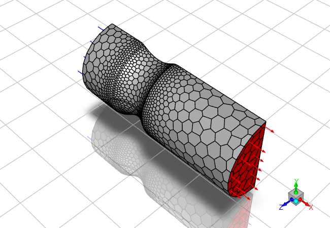
Display mesh

graphics = Graphics(solver)
mesh = Mesh(solver, new_instance_name="mesh-1")
boundary_conditions = BoundaryConditions(solver)

graphics.picture.x_resolution = 650  # Horizontal resolution for clear visualization
graphics.picture.y_resolution = 450  # Vertical resolution matching typical aspect ratio

all_walls = mesh.surfaces_list.allowed_values()

mesh.surfaces_list = all_walls
mesh.options.edges = True
mesh.display()
graphics.views.restore_view(view_name="isometric")
graphics.picture.save_picture(file_name="transient_compressible_2.png")

Configure solver

solver_general_settings = General(solver)

solver_general_settings.units.set_units(
    quantity="pressure",
    units_name="atm",
)
# density-based solver for compressible flow to capture shock behavior accurately.
solver_general_settings.solver.type = "density-based-implicit"
solver_general_settings.operating_conditions.operating_pressure = 0

setup = Setup(solver)

setup.models.energy.enabled = True
setup.materials.fluid["air"].density = {"option": "ideal-gas"}

Set boundary conditions

inlet = PressureInlet(solver, name="inlet")
outlet = PressureOutlet(solver, name="outlet")

inlet.momentum.gauge_total_pressure.value = 91192.5  # Pa
inlet.momentum.supersonic_or_initial_gauge_pressure.value = 74666.3925  # Pa

# Low turbulent intensity of 1.5% for smooth inlet flow, typical for nozzle simulations.
inlet.turbulence.turbulent_intensity = 0.015

outlet.momentum.gauge_pressure.value = 74666.3925  # Pa
outlet.turbulence.backflow_turbulent_intensity = 0.015

Set solution controls

Higher Courant number balances fast convergence and stability in density-based solver

controls = Controls(solver)
controls.courant_number = 25

Define report definition

report_definitions = ReportDefinitions(solver)


report_definitions.surface.create("mass-flow-rate")
report_definitions.surface["mass-flow-rate"] = {
    "report_type": "surface-massflowrate",
    "surface_names": ["outlet"],
}

report_files = ReportFiles(solver)
report_files.create(name="mass_flow_rate_out_rfile")
report_files["mass_flow_rate_out_rfile"] = {
    "report_defs": ["mass-flow-rate"],
    "print": True,
    "file_name": "nozzle_ss.out",
}

report_plots = ReportPlots(solver)

report_plots.create("mass_flow_rate_out_rplot")
report_plots["mass_flow_rate_out_rplot"] = {
    "report_defs": ["mass-flow-rate"],
    "print": True,
}

Steady-State Initialization and Mesh Adaptation

solver.settings.file.write_case(file_name="nozzle_steady.cas.h5")

initialize = Initialization(solver)
initialize.hybrid_initialize()

cell_register = CellRegisters(solver)

# Refinement register: Mark cells where density gradient >50% of domain average
cell_register.create(name="density_scaled_gradient_refn")
cell_register["density_scaled_gradient_refn"] = {
    "type": {
        "option": "field-value",
        "field_value": {
            "derivative": {"option": "gradient"},
            "scaling": {"option": "scale-by-global-average"},
            "option": {
                "option": "more-than",
                "more_than": 0.5,  # Threshold: >50% average
            },
            "field": "density",
        },
    }
}
# Coarsening register: Mark cells where density gradient <45% of domain average
cell_register.create(name="density_scaled_gradient_crsn")
cell_register["density_scaled_gradient_crsn"] = {
    "type": {
        "option": "field-value",
        "field_value": {
            "derivative": {"option": "gradient"},
            "scaling": {"option": "scale-by-global-average"},
            "option": {
                "option": "less-than",
                "less_than": 0.45,  # Threshold: <45% average
            },
            "field": "density",
        },
    }
}

# Define adaptation criteria: Refine if gradient is high and refinement level <2; coarsen if low
solver.settings.mesh.adapt.manual_refinement_criteria = (
    "AND(density_scaled_gradient_refn, CellRefineLevel < 2)"
)
solver.settings.mesh.adapt.manual_coarsening_criteria = "density_scaled_gradient_crsn"

solver.tui.mesh.adapt.manage_criteria.add("adaption_criteria_0")

calculation = RunCalculation(solver)
calculation.iterate(iter_count=400)

Post-processing

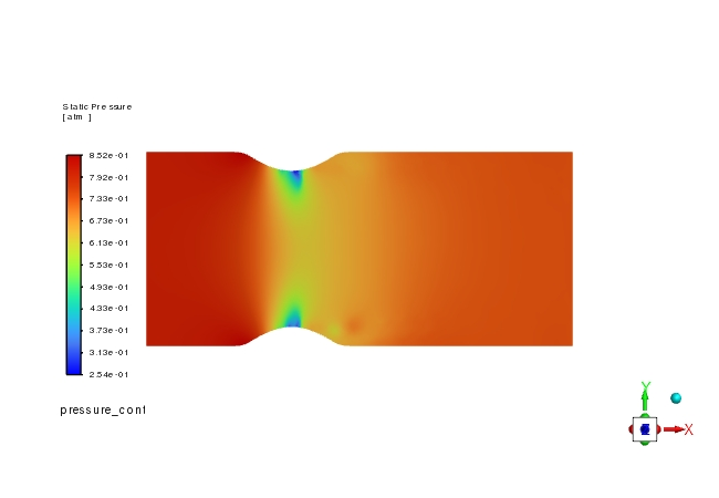
# Create pressure contour
pressure_contour = Contour(solver, new_instance_name="pressure_contour")

pressure_contour.surfaces_list = ["symmetry"]
pressure_contour.display()

graphics.views.restore_view(view_name="front")
graphics.picture.save_picture(file_name="transient_compressible_3.png")

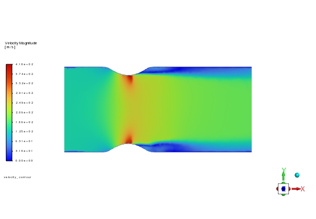
# Create velocity contour
velocity_contour = Contour(solver, new_instance_name="velocity_contour")

velocity_contour.field = "velocity-magnitude"
velocity_contour.surfaces_list = ["symmetry"]
velocity_contour.display()

graphics.views.restore_view(view_name="front")
graphics.picture.save_picture(file_name="transient_compressible_4.jpg")

# save the case and data file
solver.settings.file.write_case_data(file_name="steady_state_nozzle")

Enabling time dependence and setting transient conditions

solver_general_settings.solver.time = "unsteady-1st-order"

# Sinusoidal pressure variation at 2200 Hz simulates pulsating flow, with mean pressure of 0.737 atm.
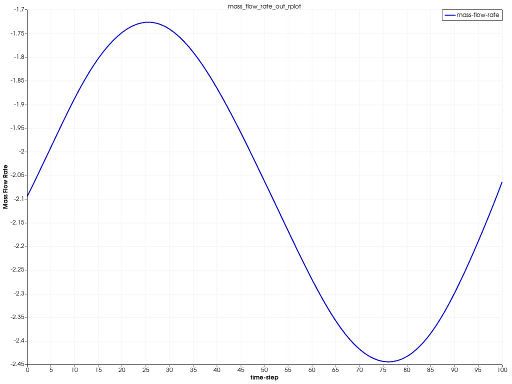
outlet.momentum.gauge_pressure.value = "(0.12*sin(2200[Hz]*t)+0.737)*101325.0[Pa]"

# Configure mesh adaptation: Refine every 25 iterations
solver.tui.mesh.adapt.manage_criteria.edit("adaption_criteria_0", "frequency", "25")

report_files["mass_flow_rate_out_rfile"] = {
    "file_name": "trans-nozzle-rfile.out",
}

report_plots["mass_flow_rate_out_rplot"].x_label = "time-step"

solver.settings.file.write_case(file_name="nozzle_unsteady.cas.h5")

Transient_controls = solver.settings.solution.run_calculation.transient_controls

Transient_controls.time_step_count = 100
Transient_controls.time_step_size = 2.85596e-05  # s: Resolves 2200 Hz oscillations
Transient_controls.max_iter_per_time_step = (
    10  # Ensures convergence within each time step
)

calculation.calculate()

mass_bal_rplot = Monitor(solver)
plot_window = GraphicsWindow()
mass_bal_rplot.monitor_set_name = "mass_flow_rate_out_rplot"
plot_window.add_plot(mass_bal_rplot)
plot_window.show()

Close Fluent

solver.exit()

Summary

In this example, we used PyFluent to model transient compressible flow in a nozzle with a sinusoidal pressure variation, simulating a realistic engineering scenario such as a jet engine or rocket propulsion system. The workflow demonstrated the use of the modern Watertight Geometry meshing, density-based solver setup, and post-processing with pressure and velocity contours. These procedures can be adapted to other compressible flow simulations, ensuring accurate modeling of shock waves and transient flow behavior.

References:

[1] Modeling Transient Compressible Flow, Ansys Fluent documentation​.