Note
Go to the end to download the full example code.
Modeling Flow Through Porous Media - Catalytic Converter#
Introduction#
Many industrial applications such as filters, catalyst beds, and packing, involve modeling the flow through porous media. This tutorial demonstrates the simulation workflow for a catalytic converter using PyFluent. The example showcases a complete workflow from geometry import through meshing to solution setup and post-processing.
This tutorial demonstrates how to do the following:
Import CAD geometry for a catalytic converter
Set up a watertight meshing workflow with local sizing controls
Generate a surface mesh
Cap inlets and outlets
Extract a fluid region
Generate a volume mesh
Configure porous media zones for the substrates with appropriate resistances.
Set up boundary conditions
Set up monitors, report definitions to track mass flow rate.
Initialize and run the simulation
Postprocessing results
Problem Description#
The system consists of a catalytic converter with the following components:
Fluid regions: Primary flow path and substrate regions
Solid regions: Catalytic substrate material with porous media properties
Sensing elements: Temperature and flow monitoring sensors
Boundary conditions: High-temperature inlet flow at 800K and 125 m/s
The simulation models heat transfer through the catalytic substrate using porous media with specified inertial and viscous resistance values.
Background#
Catalytic converters operate by passing exhaust gases through a porous substrate coated with catalytic materials. The porous media approach allows modeling of:
Pressure drop through substrate
Heat transfer between gas and solid phases
Flow distribution effects in the converter
The substrate is modeled as a porous zone with:
Porosity: 1.0 (fully open channels)
Inertial resistance: [1000, 1000, 1000] 1/m for pressure drop
Viscous resistance: [1×10⁶, 1×10⁶, 1000] 1/m² for flow resistance
Setup and Solution#
Preparation#
Launch Fluent meshing session and initialize the workflow.
import os
import platform

import ansys.fluent.core as pyfluent
from ansys.fluent.core import (
    Dimension,
    FluentMode,
    FluentVersion,
    Precision,
    UIMode,
    examples,
)
from ansys.fluent.core.solver import (  # noqa: E402
    CellZoneCondition,
    General,
    Graphics,
    Initialization,
    Materials,
    Mesh,
    Models,
    Monitor,
    PressureOutlet,
    ReportDefinitions,
    Results,
    RunCalculation,
    Scene,
    VelocityInlet,
)

# Launch meshing session
meshing = pyfluent.launch_fluent(
    product_version=FluentVersion.v252,
    mode=FluentMode.MESHING,
    ui_mode=UIMode.GUI,
    processor_count=4,
    precision=Precision.DOUBLE,
    dimension=Dimension.THREE,
)
Meshing Workflow#
Set up the watertight geometry workflow for complex multi-region geometry.
# Initialize watertight geometry workflow

workflow = meshing.workflow
workflow.InitializeWorkflow(WorkflowType=r"Watertight Geometry")
Import Geometry#
Import the catalytic converter geometry file.
# Import geometry with platform-specific file handling

filenames = {
    "Windows": "catalytic_converter.dsco",
    "Other": "catalytic_converter.dsco.pmdb",
}

geometry_filename = examples.download_file(
    filenames.get(platform.system(), filenames["Other"]),
    "/pyfluent/catalytic_converter/",
    save_path=os.getcwd(),
)

workflow.InitializeWorkflow(WorkflowType="Watertight Geometry")
workflow.TaskObject["Import Geometry"].Arguments = dict(FileName=geometry_filename)
workflow.TaskObject["Import Geometry"].Execute()
Local Sizing Controls#
Add local sizing controls for sensor components to ensure adequate mesh resolution.
# Add local sizing for sensor components

workflow.TaskObject["Add Local Sizing"].Arguments = dict(
    {
        "AddChild": "yes",
        "BOIControlName": "sensor",
        "BOIExecution": "Curvature",
        "BOIFaceLabelList": [
            "sensing_element-65-solid",
            "sensor_innertube-67-solid",
            "sensor_protectiontube-66-solid1",
        ],
        "BOIMaxSize": 1.2,
        "BOIMinSize": 0.1,
    }
)
workflow.TaskObject["Add Local Sizing"].AddChildToTask()
workflow.TaskObject["Add Local Sizing"].InsertCompoundChildTask()
workflow.TaskObject["Add Local Sizing"].Arguments = dict({"AddChild": "yes"})
workflow.TaskObject["sensor"].Execute()
Surface Mesh Generation#
Generate surface mesh with quality improvements.
# Configure surface mesh settings

workflow.TaskObject["Generate the Surface Mesh"].Arguments = dict(
    {
        "CFDSurfaceMeshControls": {"MinSize": 1.5},
        "SurfaceMeshPreferences": {
            "SMQualityImprove": "yes",
            "SMQualityImproveLimit": 0.95,
            "ShowSurfaceMeshPreferences": True,
        },
    }
)
workflow.TaskObject["Generate the Surface Mesh"].Execute()
Geometry Description#
Describe the geometry setup with fluid and solid regions requiring capping.
# Describe geometry type

workflow.TaskObject["Describe Geometry"].UpdateChildTasks(SetupTypeChanged=False)
workflow.TaskObject["Describe Geometry"].Arguments = dict(
    {"SetupType": "The geometry consists of both fluid and solid regions and/or voids"}
)
workflow.TaskObject["Describe Geometry"].UpdateChildTasks(SetupTypeChanged=True)

# Enable capping and wall-to-internal conversion

workflow.TaskObject["Describe Geometry"].Arguments = dict(
    {
        "CappingRequired": "Yes",
        "SetupType": "The geometry consists of both fluid and solid regions and/or voids",
    }
)
workflow.TaskObject["Describe Geometry"].UpdateChildTasks(SetupTypeChanged=False)
workflow.TaskObject["Describe Geometry"].Arguments = dict(
    {
        "CappingRequired": "Yes",
        "SetupType": "The geometry consists of both fluid and solid regions and/or voids",
        "WallToInternal": "Yes",
    }
)
workflow.TaskObject["Describe Geometry"].Execute()
Boundary Capping#
Create inlet and outlet boundary patches through capping operations.
# Create inlet boundary

workflow.TaskObject["Enclose Fluid Regions (Capping)"].Arguments = dict(
    {
        "LabelSelectionList": ["in1"],
        "PatchName": "inlet",
    }
)
workflow.TaskObject["Enclose Fluid Regions (Capping)"].AddChildToTask()
workflow.TaskObject["Enclose Fluid Regions (Capping)"].InsertCompoundChildTask()
workflow.TaskObject["inlet"].Execute()

# Create outlet boundary as pressure outlet

workflow.TaskObject["Enclose Fluid Regions (Capping)"].Arguments = dict(
    {
        "LabelSelectionList": ["out1"],
        "PatchName": "outlet",
    }
)
workflow.TaskObject["Enclose Fluid Regions (Capping)"].AddChildToTask()
workflow.TaskObject["Enclose Fluid Regions (Capping)"].InsertCompoundChildTask()
workflow.TaskObject["outlet"].Execute()

# Configure outlet as pressure-outlet

workflow.TaskObject["outlet"].Revert()
workflow.TaskObject["outlet"].Arguments = dict(
    {
        "CompleteLabelSelectionList": ["out1"],
        "LabelSelectionList": ["out1"],
        "PatchName": "outlet",
        "ZoneType": "pressure-outlet",
    }
)
workflow.TaskObject["outlet"].Execute()

# Update boundaries

workflow.TaskObject["Update Boundaries"].Execute()
Region Setup#
Create and configure fluid regions including substrate conversion.
# Create multiple flow volumes

workflow.TaskObject["Create Regions"].Arguments = dict({"NumberOfFlowVolumes": 3})
workflow.TaskObject["Create Regions"].Execute()

# Convert solid substrate regions to fluid regions

workflow.TaskObject["Update Regions"].Arguments = dict(
    {
        "OldRegionNameList": ["honeycomb-solid1", "honeycomb_af0-solid1"],
        "OldRegionTypeList": ["solid", "solid"],
        "RegionNameList": ["fluid:substrate:1", "fluid:substrate:2"],
        "RegionTypeList": ["fluid", "fluid"],
    }
)
workflow.TaskObject["Update Regions"].Execute()
Boundary Layer Mesh#
Add boundary layer mesh for accurate near-wall resolution.
# Add boundary layers

workflow.TaskObject["Add Boundary Layers"].AddChildToTask()
workflow.TaskObject["Add Boundary Layers"].InsertCompoundChildTask()
workflow.TaskObject["smooth-transition_1"].Arguments = dict(
    {"BLControlName": "smooth-transition_1"}
)

workflow.TaskObject["smooth-transition_1"].Execute()
Volume Mesh Generation#
Generate the final volume mesh with body label merging.
# Generate volume mesh

workflow.TaskObject["Generate the Volume Mesh"].Arguments = dict(
    {"VolumeMeshPreferences": {"MergeBodyLabels": "yes"}}
)
workflow.TaskObject["Generate the Volume Mesh"].Execute()
Mesh Quality Check & Write Mesh File#
Check mesh quality and write mesh files and snapshot.
# Check mesh quality

meshing.tui.mesh.check_mesh()

# Write mesh files

meshing.tui.file.write_mesh("out/catalytic_converter.msh.h5")
Switch to Solver#
Switch from meshing to solver mode for setup and solution.
# Switch to solver mode

solver_session = meshing.switch_to_solver()
# Visualize mesh in the graphics window and save a screenshot
# Create Graphics object to save the graphics with following settings

graphics = Graphics(solver_session)
graphics.views.auto_scale()
if graphics.picture.use_window_resolution.is_active():
    graphics.picture.use_window_resolution = False

graphics.views.restore_view(view_name="isometric")
graphics.picture.x_resolution = 600
graphics.picture.y_resolution = 600
graphics.picture.color_mode = "color"

# Define and display the mesh
# First, get all wall boundary names and create a mesh object for visualization context

all_walls = solver_session.settings.setup.boundary_conditions.wall.get_object_names()
mesh = Mesh(solver_session, new_instance_name="mesh-1")
mesh.surfaces_list = all_walls
mesh.options.edges = True
mesh.display()
os.makedirs("out", exist_ok=True)
graphics.picture.save_picture(file_name="out/catalytic_converter_mesh.png")
mesh.options.edges = False  # Turn off edges after saving the picture
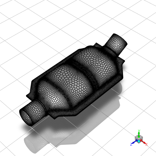
Polyhedra mesh for the catalytic converter geometry.#
General Setup#
Configure units and enable energy equation.
# Set length units to millimeters

general_settings = General(solver_session)
general_settings.units_settings.new_unit(
    offset=0.0, units_name="mm", scale_factor=1.0, quantity="length"
)
# Enable energy equation
energy_model_settings = Models(solver_session)
energy_model_settings.energy = {
    "enabled": True,
    "inlet_diffusion": False,
}
Materials#
Set up material properties for the fluid.
# Copy nitrogen from database

solver_session.settings.setup.materials.database.copy_by_name(
    type="fluid", name="nitrogen"
)

# Assign material to main fluid zone

materials = Materials(solver_session)
materials.database.copy_by_name(type="fluid", name="nitrogen")

material_assignments = CellZoneCondition(solver_session, name="fluid:1")
material_assignments.general = {"material": "nitrogen"}

# Copy boundary conditions to other fluid zones

solver_session.tui.define.boundary_conditions.copy_bc(
    "fluid:1", "fluid:2", "fluid:3", "()"
)
Cell Zone Conditions#
Configure porous media properties for catalytic substrate zones.
# Configure first substrate zone as porous media

porous_media_settings = CellZoneCondition(solver_session, name="fluid:substrate:1")
porous_media_settings.general = {"laminar": True, "material": "nitrogen"}
porous_media_settings.porous_zone = {
    "solid_material": "aluminum",
    "equib_thermal": True,
    "relative_viscosity": {"value": 1, "option": "constant"},
    "porosity": 1,
    "power_law_model": [0, 0],
    "inertial_resistance": [1000.0, 1000.0, 1000.0],
    "alt_inertial_form": False,
    "viscous_resistance": [1000000.0, 1000000.0, 1000.0],
    "rel_vel_resistance": True,
    "direction_2_vector": [0, 1, 0],
    "direction_1_vector": [1, 0, 0],
    "dir_spec_cond": "Cartesian",
    "porous": True,
}


# Copy porous media settings to second substrate zone

solver_session.tui.define.boundary_conditions.copy_bc(
    "fluid:substrate:1", "fluid:substrate:2", "()"
)
Boundary Conditions#
Set up inlet and outlet boundary conditions.
# Configure velocity inlet

velocity_inlet = VelocityInlet(solver_session, name="inlet")
velocity_inlet.momentum = {"velocity_magnitude": {"value": 125.0}}

velocity_inlet.turbulence = {
    "hydraulic_diameter": 0.5,  # in meters
    "turbulence_specification": "Intensity and Hydraulic Diameter",
}
velocity_inlet.thermal = {"temperature": {"value": 800.0}}  # in Kelvin

# Configure pressure outlet

pressure_outlet = PressureOutlet(solver_session, name="outlet")
pressure_outlet.momentum = {"gauge_pressure": {"value": 0.0}}
pressure_outlet.turbulence = {
    "backflow_hydraulic_diameter": 0.5,  # in meters
    "turbulence_specification": "Intensity and Hydraulic Diameter",
}
pressure_outlet.thermal = {"backflow_total_temperature": {"value": 800.0}}  # in Kelvin
Solution Monitoring#
Set up surface monitors for mass flow rate tracking.
# Create surface report definition

report_definitions = ReportDefinitions(solver_session)
surface_report = report_definitions.surface.create(name="surf-mon-1")
surface_report.report_type = "surface-massflowrate"
surface_report.surface_names = ["outlet"]

# Create report file monitor

monitor = Monitor(solver_session)
surface_monitor = monitor.report_files.create(name="surf-mon-1")
surface_monitor.print = True
surface_monitor.report_defs = ["surf-mon-1"]
os.makedirs("out", exist_ok=True)
surface_monitor.file_name = "out/surf-mon-1.out"

# Create report plot monitor

surface_plot_monitor = monitor.report_plots.create(name="surf-mon-1")
surface_plot_monitor.print = True
surface_plot_monitor.report_defs = ["surf-mon-1"]
Initialization#
Initialize the flow field.
# Compute initial conditions from inlet

solution_initialization = Initialization(solver_session)

solution_initialization.compute_defaults(
    from_zone_type="velocity-inlet", from_zone_name="inlet", phase="mixture"
)

# Set initialization method and initialize

solution_initialization.initialization_type = "standard"
solution_initialization.standard_initialize()
Run Calculation#
Execute the iterative solution process.
# Set iteration count and run calculation

run_calculation = RunCalculation(solver_session)
run_calculation.iter_count = (
    150  # Iteration count, keep it at 150 for demo purposes only
)
run_calculation.calculate()
Results Processing#
Extract and analyze simulation results.
# Mass Flow Analysis
# ~~~~~~~~~~~~~~~~~~
# Calculate mass flow rate at outlet.

# Ensure the 'out/' directory exists before writing files to it
os.makedirs("out", exist_ok=True)
results = Results(solver_session)
results.report.fluxes.mass_flow(
    zones=["outlet"], write_to_file=True, file_name="out/mass_flow_rate.flp"
)
Surface Creation#
Create iso-surfaces for flow field visualization.
# Create cross-sectional surfaces

surfaces_data = [
    ("y=-425", "y-coordinate", [-0.425]),
    ("z=185", "z-coordinate", [0.185]),
    ("z=230", "z-coordinate", [0.23]),
    ("z=280", "z-coordinate", [0.28]),
    ("z=330", "z-coordinate", [0.33]),
    ("z=375", "z-coordinate", [0.375]),
]

for surf_name, field_name, iso_values in surfaces_data:
    results.surfaces.iso_surface.create(name=surf_name)
    results.surfaces.iso_surface[surf_name].field = field_name
    results.surfaces.iso_surface[surf_name].iso_values = iso_values
Velocity Analysis#
Calculate mass-weighted average velocity at different axial locations.
z_surfaces = ["z=185", "z=230", "z=280", "z=330", "z=375"]
results.report.surface_integrals.mass_weighted_avg(
    surface_names=z_surfaces,
    report_of="velocity-magnitude",
    write_to_file=True,
    file_name="out/mass-avg_vel.srp",
)
Vector Plot#
Create velocity vector, static pressure, and velocity magnitude plots.
This section demonstrates post-processing visualization techniques using PyFluent’s graphics capabilities. We’ll create three different types of visualizations:
Velocity Vectors: Show flow direction and magnitude using vectors
Static Pressure Contours: Display pressure distribution along a cross-section
Velocity Magnitude Contours: Visualize velocity distribution across multiple surfaces
Each visualization is displayed in a separate scene with consistent mesh transparency to provide context and better understanding of the flow field.
# Create velocity vector plot
# Velocity vectors show both flow direction and magnitude using arrow symbols
# The scale factor controls arrow size for optimal visualization

results.graphics.vector.create(name="vector-vel")
results.graphics.vector["vector-vel"] = {
    "scale": {
        "auto_scale": True,  # Automatically scale arrows for best visibility
        "scale_f": 0.006,  # Fine-tune scale factor (smaller = shorter arrows)
    },
    "surfaces_list": ["y=-425"],  # Display vectors on the y=-425 cross-section
}

# Create static pressure contour plot
# Pressure contours use color mapping to show pressure distribution
# This helps identify high/low pressure regions and pressure gradients

results.graphics.contour.create(name="contour-ps")
results.graphics.contour["contour-ps"] = {
    "field": "pressure",  # Specify pressure as the contour variable
    "surfaces_list": ["y=-425"],  # Display on the same cross-section as vectors
}

# Create velocity magnitude contour plot
# Velocity magnitude shows speed distribution without directional information
# Using multiple z-surfaces provides a comprehensive view through the domain

results.graphics.contour.create(name="contour-velmag")
results.graphics.contour["contour-velmag"] = {
    "field": "velocity-magnitude",  # Specify velocity magnitude as the variable
    "surfaces_list": z_surfaces,  # Display on all z-coordinate surfaces
}

# Scene 1: Display velocity vectors with mesh context
# Scenes combine multiple graphics objects for comprehensive visualization

velocity_vectors_scene = Scene(solver_session, new_instance_name="scene-1")
velocity_vectors_scene.graphics_objects.add(name="vector-vel")

# adding mesh for context which is created earlier steps just after switching to solver

velocity_vectors_scene.graphics_objects.add(name="mesh-1")

# Configure scene appearance and display settings
solver_session.settings.results.scene["scene-1"] = {
    "graphics_objects": {
        "vector-vel": {"name": "vectors"},  # Label for the vector plot
        "mesh-1": {"transparency": 75},  # Semi-transparent mesh (75% transparent)
    }
}
velocity_vectors_scene.display()
graphics.views.auto_scale()
os.makedirs("out", exist_ok=True)
graphics.picture.save_picture(file_name="out/velocity_vectors.png")
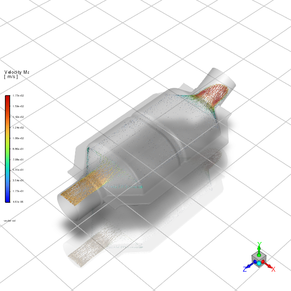
Velocity Vectors Through the Interior#
# Scene 2: Display static pressure contours with mesh context
# This scene focuses on pressure distribution across the catalytic converter

static_pressure_scene = Scene(solver_session, new_instance_name="scene-2")
static_pressure_scene.graphics_objects.add(name="contour-ps")
static_pressure_scene.graphics_objects.add(name="mesh-1")

# Configure pressure contour scene settings

solver_session.settings.results.scene["scene-2"] = {
    "graphics_objects": {
        "contour-ps": {"name": "contour-ps"},  # Label for the pressure contour
        "mesh-1": {"transparency": 75},  # Consistent mesh transparency
    }
}
static_pressure_scene.display()
graphics.views.auto_scale()
# Ensure "out/" directory exists before saving files
os.makedirs("out", exist_ok=True)
graphics.picture.save_picture(file_name="out/static_pressure.png")
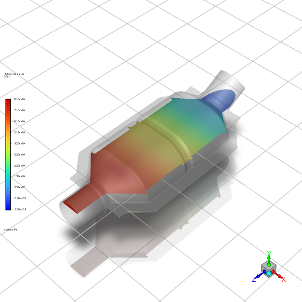
Contours of Static Pressure Through the Interior#
# Scene 3: Display velocity magnitude contours with mesh context
# This scene shows speed distribution across multiple axial locations

velocity_magnitude_scene = Scene(solver_session, new_instance_name="scene-3")
velocity_magnitude_scene.graphics_objects.add(name="contour-velmag")
velocity_magnitude_scene.graphics_objects.add(name="mesh-1")

# Configure velocity magnitude contour scene settings
solver_session.settings.results.scene["scene-3"] = {
    "graphics_objects": {
        "contour-velmag": {
            "name": "contour-velmag"
        },  # Label for velocity magnitude contour
        "mesh-1": {"transparency": 75},  # Consistent mesh transparency
    }
}
velocity_magnitude_scene.display()
graphics.views.auto_scale()
# Ensure the 'out/' directory exists before saving files
os.makedirs("out", exist_ok=True)
graphics.picture.save_picture(file_name="out/velocity_magnitude.png")
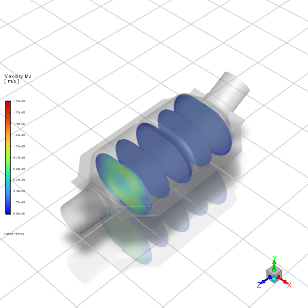
Contours of Velocity Magnitude on the z=185, z=230, z=280, z=330, and z=375 Surfaces#
File Output#
Save final case and data files.
# Write final case and data

solver_session.settings.file.write(
    file_type="case-data", file_name="out/catalytic_converter_final.cas.h5"
)
Solver Exit#
Display simulation statistics and completion message.
# Close solver session

solver_session.exit()