Note

Go to the end to download the full example code.

Simulating a 1P3S Battery Pack Using the Battery Model#

Objective#

This example demonstrates a complete 1P3S battery pack simulation workflow comprising one parallel string and three cells in series using the NTGK (Newman-Tiedemann-Gu-Kim) electrochemical model utilizing PyFluent APIs. The goal is to model and analyze battery pack behavior under a constant 200 W discharge condition. This includes setting up active and passive zones, defining dual-path electrical conductivity using User-Defined Scalars (UDS), and applying convection cooling to simulate heat dissipation. The simulation aims to monitor key performance indicators such as pack voltage, maximum temperature, current flow, and heat generation over a 1500 second transient run, providing insights into thermal and electrical performance relevant to electric vehicle (EV) and energy storage system (ESS) design.

Problem Description#

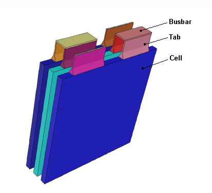
Simulation of a 1P3S lithium-ion battery pack, consisting of three cells connected in series and no parallel branches, undergoing a constant 200 W discharge to represent a high-load condition. Each cell has a nominal capacity of 14.6 Ah, resulting in a total pack capacity of 14.6 Ah and a nominal voltage range of 10.8–12.6 V, corresponding to an average cell voltage of approximately 3.9 V. The discharge C-rate equates to about 1.17C, and the total energy of roughly 171 Wh means the discharge would last around 51 minutes (3060 seconds). The simulation model includes active zones for the electrochemical cells and passive zones representing conductive components such as tabs and busbars, with defined electrical and thermal material properties. The model also incorporates natural convection cooling with a heat transfer coefficient of 5 W/m²·K and an ambient temperature of 300 K, allowing for realistic thermal management analysis.

Import modules#

Note

Importing the following classes offers streamlined access to key solver settings, eliminating the need to manually browse through the full hierarchy of settings APIs structure.

import os

import ansys.fluent.core as pyfluent
from ansys.fluent.core import examples
from ansys.fluent.core.solver import (
    Battery,
    BoundaryConditions,
    CellZoneConditions,
    Contour,
    Controls,
    General,
    Graphics,
    Initialization,
    Materials,
    Mesh,
    ReportDefinitions,
    RunCalculation,
    Solution,
    Vector,
)
from ansys.fluent.visualization import GraphicsWindow, Monitor

Launch Fluent in solver mode#

solver = pyfluent.launch_fluent(
    precision=pyfluent.Precision.DOUBLE,
    mode=pyfluent.FluentMode.SOLVER,
)

Read mesh#

mesh_file = examples.download_file(
    "1P3S_battery_pack.msh",
    "pyfluent/battery_pack",
    save_path=os.getcwd(),
)

solver.settings.file.read_mesh(file_name=mesh_file)

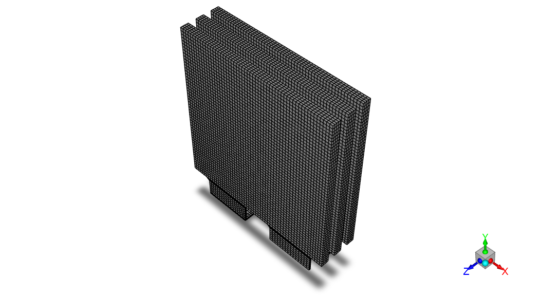
Display mesh#

graphics = Graphics(solver)
mesh = Mesh(solver, new_instance_name="mesh-1")

all_walls = mesh.surfaces_list.allowed_values()

graphics.picture.x_resolution = 650  # Horizontal resolution for clear visualization
graphics.picture.y_resolution = 450  # Vertical resolution matching typical aspect ratio

mesh.surfaces_list = all_walls
mesh.options.edges = True
mesh.display()

graphics.picture.save_picture(file_name="battery_pack_1.png")

Solver settings#

solver_general_settings = General(solver)

solver_general_settings.solver.time = "unsteady-1st-order"

Enable Battery Model (NTGK/DCIR)#

Note

Using wildcards (*, ?, |, etc.) instead of explicit zone lists makes the setup more flexible and scalable. For example:

cell_* → selects all zones starting with cell_ (e.g., cell_1, cell_2, …)
*bar*|*tabzone* → selects zones containing either bar or tabzone (e.g., bar1, n_tabzone_1,…)

battery_model = Battery(solver)

battery_model.enabled = True
battery_model.echem_model = "ntgk/dcir"
battery_model.eload_condition.eload_settings.eload_type = "specified-system-power"
battery_model.eload_condition.eload_settings.power_value = 200  # W  (Total pack power)

# Conductive zones
battery_model.zone_assignment.active_zone = "cell_*"  # Active cells
battery_model.zone_assignment.passive_zone = "*bar*|*tabzone*"  # Bars zones + tab zones

# External electrical contacts
battery_model.zone_assignment.negative_tab = ["tab_n"]  # Negative terminal
battery_model.zone_assignment.positive_tab = ["tab_p"]  # Positive terminal

Define materials#

materials = Materials(solver)

# Active material (cells): conductivity via UDS-0 and UDS-1
materials.solid.create("e_material")

materials.solid["e_material"] = {
    "chemical_formula": "e",
    "thermal_conductivity": {"value": 20},  # W/(m·K)
    "uds_diffusivity": {
        "option": "defined-per-uds",
        "uds_diffusivities": {
            "uds-0": {"value": 1000000},  # S/m  (Electronic conductivity)
            "uds-1": {"value": 1000000},  # S/m  (Ionic conductivity)
        },
    },
}

# Passive material (busbars & tabs): high constant conductivity
materials.solid.create("busbar_material")

materials.solid["busbar_material"] = {
    "chemical_formula": "bus",
    "uds_diffusivity": {
        "option": "value",
        "value": 3.541e7,  # S/m  (Copper-like conductivity)
    },
}

Assign materials to cell zones#

cell_zone_conditions = CellZoneConditions(solver)

# Assign e_material to cell_1
cell_zone_conditions.solid["cell_1"] = {"general": {"material": "e_material"}}

# Copy to cell_2 and cell_3
cell_zone_conditions.copy(from_="cell_1", to="cell_*")

# Assign busbar_material to bar1
cell_zone_conditions.solid["bar1"] = {"general": {"material": "busbar_material"}}

# Copy to all passive zones
cell_zone_conditions.copy(from_="bar1", to="*bar*|*tabzone*")
# '*bar*' matches any zone containing 'bar',
# '|*tabzone*' matches any zone containing 'tabzone' → OR logic

Boundary conditions#

conditions = BoundaryConditions(solver)

# Convection on wall-cell_1
conditions.wall["wall-cell_1"] = {
    "thermal": {
        "thermal_condition": "Convection",
        "heat_transfer_coeff": {"value": 5},  # W/(m²·K)
    }
}

# Copy to all other walls (tabs, busbars, cells)
conditions.copy(from_="wall-cell_1", to="wall*")

Define solution controls and monitors#

controls = Controls(solver)

# Disable flow and turbulence equations
controls.equations = {
    "flow": False,
    "kw": False,
}

solution = Solution(solver)

solution.monitor.residual.options.criterion_type = (
    "none"  # No automatic convergence check
)

Define report definitions#

definitions = ReportDefinitions(solver)

# Surface report: voltage at positive tab (area-weighted average)
definitions.surface["voltage_surface_areaavg"] = {
    "report_type": "surface-areaavg",
    "field": "passive-zone-potential",
    "surface_names": ["tab_p"],
    "create_report_file": True,
    "create_report_plot": True,
}

# Format plot axes
report_plot = solver.settings.solution.monitor.report_plots[
    "voltage_surface_areaavg-rplot"
]
report_plot.axes.x.number_format.precision = 0  # Integer time steps
report_plot.axes.y.number_format.precision = 2  # 2 decimal places for voltage

# Volume report: maximum temperature in all cell zones
definitions.volume["volume_max_temp"] = {
    "report_type": "volume-max",
    "field": "temperature",
    "cell_zones": "*cell|*bar*|*tabzone*",
    "create_report_file": True,
    "create_report_plot": True,
}

# Format plot axes
report_plot_1 = solver.settings.solution.monitor.report_plots["volume_max_temp-rplot"]
report_plot_1.axes.x.number_format.precision = 0
report_plot_1.axes.y.number_format.precision = 2

Initialize solution#

initialize = Initialization(solver)
initialize.standard_initialize()

Transient controls#

Transient_controls = solver.settings.solution.run_calculation.transient_controls

Transient_controls.time_step_count = 50  # Number of time steps
Transient_controls.time_step_size = 30  # s  (30 s per step)

calculation = RunCalculation(solver)
calculation.calculate()  # Run transient simulation

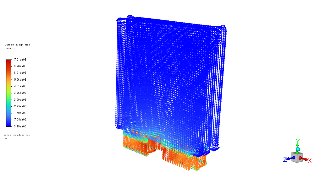
Post-processing#

# Current density vector plot
vector = Vector(solver, new_instance_name="current-magnitude-vector")

vector.vector_field = "current-density-j"  # A/m²  (Current density vector)
vector.field = "current-magnitude"  # A/m²  (Magnitude for coloring)
vector.surfaces_list = ["tab_n", "tab_p", "wall*"]
vector.options.vector_style = "arrow"
vector.options.scale = 0.03  # Scale factor for visibility
vector.vector_opt.fixed_length = True  # Uniform arrow length
vector.display()

graphics.views.restore_view(view_name="isometric")
graphics.picture.save_picture(file_name="battery_pack_2.png")

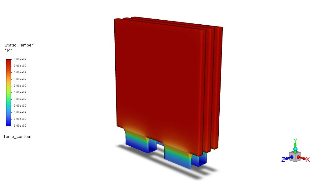
# Temperature contour
temp_contour = Contour(solver, new_instance_name="temp_contour")

temp_contour.field = "temperature"  # K
temp_contour.surfaces_list = ["tab_n", "tab_p", "wall*"]
temp_contour.colorings.banded = True
temp_contour.display()

graphics.views.restore_view(view_name="isometric")
graphics.picture.save_picture(file_name="battery_pack_3.png")

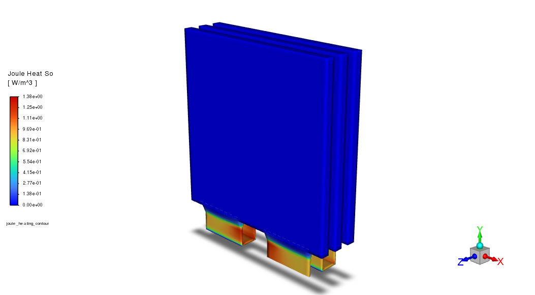
# Joule heat source contour
joule_contour = Contour(solver, new_instance_name="joule_heating_contour")

joule_contour.field = "battery-joule-heat-source"  # W/m³
joule_contour.surfaces_list = ["tab_n", "tab_p", "wall*"]
joule_contour.colorings.banded = True
joule_contour.display()

graphics.views.restore_view(view_name="isometric")
graphics.picture.save_picture(file_name="battery_pack_4.png")

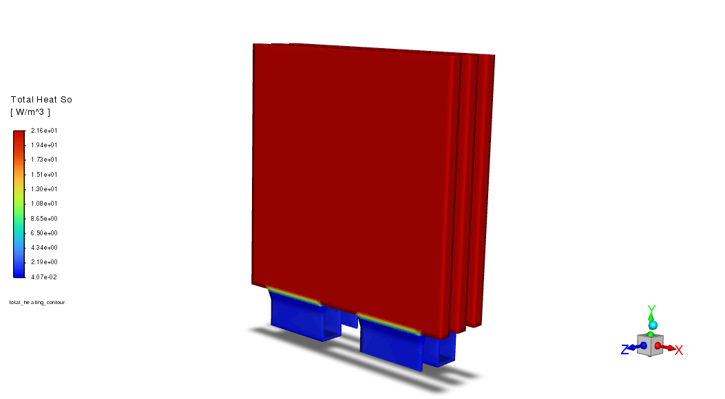
# Total heat source contour
total_heat_contour = Contour(solver, new_instance_name="total_heating_contour")

total_heat_contour.field = "total-heat-source"  # W/m³  (Joule + reaction heat)
total_heat_contour.surfaces_list = ["tab_n", "tab_p", "wall*"]
total_heat_contour.colorings.banded = True
total_heat_contour.display()

graphics.views.restore_view(view_name="isometric")
graphics.picture.save_picture(file_name="battery_pack_5.png")

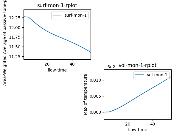
Display monitor plots#

plot_window = GraphicsWindow(solver)

voltage_rplot = Monitor(solver, monitor_set_name="voltage_surface_areaavg-rplot")
plot_window.add_plot(voltage_rplot, position=(0, 0))

temp_rplot = Monitor(solver, monitor_set_name="volume_max_temp-rplot")
plot_window.add_plot(temp_rplot, position=(1, 1))

plot_window.renderer = "matplotlib"
plot_window.show()

Save case and data#

solver.settings.file.write_case_data(file_name="1P3S_Battery_Pack")

Close Fluent#

solver.exit()

Summary#

This example provides a complete and reproducible PyFluent workflow for simulating a multi-cell battery pack using the Battery Model with the NTGK sub-model. It demonstrates how to set up active and passive zones, apply constant power discharge, use UDS-based dual-path conductivity, and monitor voltage and temperature behavior during operation. It serves as a template for battery pack analysis, applicable to designs ranging from small modules to full EV packs.

References:#

[1] Simulating a 1P3S Battery Pack Using the Battery Model, Ansys Fluent documentation.

Gallery generated by Sphinx-Gallery