Modeling External Compressible Flow

The purpose of this tutorial is to compute the turbulent flow past a transonic wing at a nonzero angle of attack using the k-w SST turbulence model.

This example uses the guided workflow for watertight geometry meshing because it is appropriate for geometries that can have no imperfections, such as gaps and leakages.

Workflow tasks

The Modeling External Compressible Flow Using the Meshing Workflow guides you through these tasks:

• Creation of capsule mesh using Watertight Geometry workflow.

• Model compressible flow (using the ideal gas law for density).

• Set boundary conditions for external aerodynamics.

• Use the k-w SST turbulence model.

• Calculate a solution using the pressure-based coupled solver with global time step selected for the pseudo time method.

• Check the near-wall mesh resolution by plotting the distribution of .

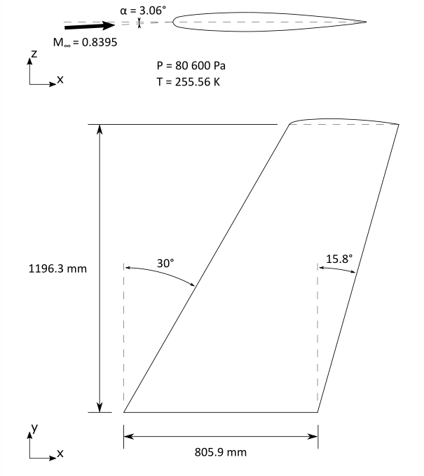
Problem description

The problem considers the flow around a wing at an angle of attack a=3.06° and a free stream Mach number of 0.8395 (M=0.8395). The flow is transonic, and has a shock near the mid-chord (x/c≃0.20) on the upper (suction) side. The wing has a mean aerodynamic chord length of 0.64607 m, a span of 1.1963 m, an aspect ratio of 3.8, and a taper ratio of 0.562.

Example Setup

Before you can use the meshing workflow, you must set up the example and initialize this workflow.

Perform required imports

Perform required imports, which includes downloading and importing the geometry files.

import ansys.fluent.core as pyfluent
from ansys.fluent.core import examples

wing_spaceclaim_file, wing_intermediary_file = [
    examples.download_file(CAD_file, "pyfluent/external_compressible")
    for CAD_file in ["wing.scdoc", "wing.pmdb"]
]

Download successful. File path:
/home/ansys/.local/share/ansys_fluent_core/examples/wing.scdoc
Download successful. File path:
/home/ansys/.local/share/ansys_fluent_core/examples/wing.pmdb

Launch Fluent

Launch Fluent as a service in meshing mode with double precision running on four processors.

meshing = pyfluent.launch_fluent(
    precision="double",
    processor_count=4,
    mode="meshing",
)

Initialize workflow

Initialize the watertight geometry meshing workflow.

meshing.workflow.InitializeWorkflow(WorkflowType="Watertight Geometry")

Watertight geometry meshing workflow

The fault-tolerant meshing workflow guides you through the several tasks that follow.

Import CAD and set length units

Import the CAD geometry and set the length units to inches.

geo_import = meshing.workflow.TaskObject["Import Geometry"]
geo_import.Arguments.set_state(
    {
        "FileName": wing_intermediary_file,
    }
)

geo_import.Execute()

Add local sizing

Add local sizing controls to the faceted geometry.

local_sizing = meshing.workflow.TaskObject["Add Local Sizing"]
local_sizing.Arguments.set_state(
    {
        "AddChild": "yes",
        "BOIControlName": "wing-facesize",
        "BOIFaceLabelList": ["wing_bottom", "wing_top"],
        "BOISize": 10,
    }
)

local_sizing.AddChildAndUpdate()

local_sizing.Arguments.set_state(
    {
        "AddChild": "yes",
        "BOIControlName": "wing-ege-facesize",
        "BOIFaceLabelList": ["wing_edge"],
        "BOISize": 2,
    }
)

local_sizing.AddChildAndUpdate()

local_sizing.Arguments.set_state(
    {
        "AddChild": "yes",
        "BOIControlName": "boi_1",
        "BOIExecution": "Body Of Influence",
        "BOIFaceLabelList": ["wing-boi"],
        "BOISize": 5,
    }
)

local_sizing.AddChildAndUpdate()

Generate surface mesh

Generate the surface mash.

surface_mesh_gen = meshing.workflow.TaskObject["Generate the Surface Mesh"]
surface_mesh_gen.Arguments.set_state(
    {"CFDSurfaceMeshControls": {"MaxSize": 1000, "MinSize": 2}}
)

surface_mesh_gen.Execute()

Describe geometry

Describe geometry and define the fluid region.

describe_geo = meshing.workflow.TaskObject["Describe Geometry"]
describe_geo.UpdateChildTasks(SetupTypeChanged=False)

describe_geo.Arguments.set_state(
    {"SetupType": "The geometry consists of only fluid regions with no voids"}
)

describe_geo.UpdateChildTasks(SetupTypeChanged=True)

describe_geo.Execute()

Update boundaries

Update the boundaries.

meshing.workflow.TaskObject["Update Boundaries"].Execute()

Update regions

Update the regions.

meshing.workflow.TaskObject["Update Regions"].Execute()

Add boundary layers

Add boundary layers, which consist of setting properties for the boundary layer mesh.

add_boundary_layer = meshing.workflow.TaskObject["Add Boundary Layers"]
add_boundary_layer.Arguments.set_state({"NumberOfLayers": 12})

add_boundary_layer.AddChildAndUpdate()

Generate volume mesh

Generate the volume mesh, which consists of setting properties for the volume mesh.

volume_mesh_gen = meshing.workflow.TaskObject["Generate the Volume Mesh"]
volume_mesh_gen.Arguments.set_state(
    {
        "VolumeFill": "poly-hexcore",
        "VolumeFillControls": {"HexMaxCellLength": 512},
        "VolumeMeshPreferences": {
            "CheckSelfProximity": "yes",
            "ShowVolumeMeshPreferences": True,
        },
    }
)

volume_mesh_gen.Execute()

Check mesh in meshing mode

Check the mesh in meshing mode.

meshing.tui.mesh.check_mesh()

Save mesh file

Save the mesh file (wing.msh.h5).

meshing.tui.file.write_mesh("wing.msh.h5")

Solve and postprocess

Once you have completed the watertight geometry meshing workflow, you can solve and postprcess the results.

Switch to solution mode

Switch to solution mode. Now that a high-quality mesh has been generated using Fluent in meshing mode, you can switch to solver mode to complete the setup of the simulation.

solver = meshing.switch_to_solver()

Check mesh in solver mode

Check the mesh in solver mode. The mesh check lists the minimum and maximum x, y, and z values from the mesh in the default SI units of meters. It also reports a number of other mesh features that are checked. Any errors in the mesh are reported.

solver.mesh.check()

Define model

Set the k-w sst turbulence model.

# model : k-omega
# k-omega model : sst

viscous = solver.setup.models.viscous

viscous.model = "k-omega"
viscous.k_omega_model = "sst"

Define materials

Modify the default material air to account for compressibility and variations of the thermophysical properties with temperature.

# density : ideal-gas
# viscosity : sutherland
# viscosity method : three-coefficient-method
# reference viscosity : 1.716e-05 [kg/(m s)]
# reference temperature : 273.11 [K]
# effective temperature : 110.56 [K]

air = solver.setup.materials.fluid["air"]

air.density.option = "ideal-gas"

air.viscosity.option = "sutherland"

air.viscosity.sutherland.option = "three-coefficient-method"

air.viscosity.sutherland.reference_viscosity = 1.716e-05

air.viscosity.sutherland.reference_temperature = 273.11

air.viscosity.sutherland.effective_temperature = 110.56

Boundary Conditions

Set the boundary conditions for pressure_farfield.

# gauge pressure : 0 [Pa]
# mach number : 0.8395
# temperature : 255.56 [K]
# x-component of flow direction : 0.998574
# z-component of flow direction : 0.053382
# turbulent intensity : 5 [%]
# turbulent viscosity ratio : 10

pressure_farfield = solver.setup.boundary_conditions.pressure_far_field[
    "pressure_farfield"
]

pressure_farfield.gauge_pressure = 0

pressure_farfield.m = 0.8395

pressure_farfield.t = 255.56

pressure_farfield.flow_direction[0] = 0.998574

pressure_farfield.flow_direction[2] = 0.053382

pressure_farfield.turbulent_intensity = 0.05

pressure_farfield.turbulent_viscosity_ratio_real = 10

Operating Conditions

Set the operating conditions.

# operating pressure : 80600 [Pa]

solver.setup.general.operating_conditions.operating_pressure = 80600

Initialize flow field

Initialize the flow field using hybrid initialization.

solver.solution.initialization.hybrid_initialize()

Save case file

Save the case file external_compressible1.cas.h5.

solver.file.write(file_name="external_compressible.cas.h5", file_type="case")

Solve for 25 iterations

Solve for 25 iterations (100 iterations is recommended, however for this example 25 is sufficient).

solver.solution.run_calculation.iterate(iter_count=25)

Write final case file and data

Write the final case file and the data.

solver.file.write(file_name="external_compressible1.cas.h5", file_type="case")

Close Fluent

Close Fluent.

solver.exit()