Note
Go to the end to download the full example code.
Modeling Solidification#
Objective#
This example models solidification in a Czochralski crystal growth process using PyFluent. The simulation involves setting up a two-dimensional axisymmetric swirl configuration with gravity and activating the Solidification and Melting model to capture phase change behavior. Pull velocities are applied to represent continuous casting, while Marangoni convection is incorporated through a surface tension gradient at the melt surface. The workflow begins with a steady state conduction solution to establish a realistic initial thermal field. Subsequently, transient flow and heat transfer are enabled to capture the combined effects of natural and Marangoni convection. To achieve this, custom field functions and patching techniques are employed for efficient definition of pull velocities and initialization of the simulation.
Problem Description#
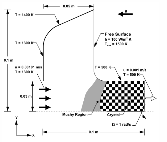
The problem involves simulating a two-dimensional axisymmetric bowl containing liquid metal. The liquid enters from the bottom at a temperature of 1300 K, while solidified material is continuously pulled from the top at a rate of 0.001 m/s. The crystal undergoes rotation at an angular velocity of 1 rad/s, which induces a swirling flow within the melt. Heat loss from the upper region of the crystal promotes solidification of the liquid metal. Additionally, Marangoni convection develops at the free surface due to temperature-dependent variations in surface tension. The solidification process is modeled with zero mushy zone width, where both the solidus and liquidus temperatures are 1150 K. The flow incorporates an axial pull velocity of 0.001 m/s and a swirl velocity defined by ω × r, with ω = 1 rad/s. The surface tension gradient responsible for Marangoni stress is given by dσ/dT = –0.00036 N/m·K, and gravity acts in the axial (X) direction with a magnitude of –9.81 m/s².
Import modules#
Note
Importing the following classes offer streamlined access to key solver settings, eliminating the need to manually browse through the full settings structure.
import os

import ansys.fluent.core as pyfluent
from ansys.fluent.core import examples
from ansys.fluent.core.solver import (
    BoundaryConditions,
    Contour,
    Controls,
    General,
    Graphics,
    Initialization,
    Materials,
    Mesh,
    Methods,
    Results,
    RunCalculation,
    Setup,
    Solution,
    VelocityInlet,
)
Launch Fluent session in solver mode#
solver = pyfluent.launch_fluent(
    precision=pyfluent.Precision.DOUBLE,
    mode="solver",
    dimension=pyfluent.Dimension.TWO,
)
Download mesh file#
mesh_file = examples.download_file(
    "solid.msh",
    "pyfluent/solidification",
    save_path=os.getcwd(),
)

solver.settings.file.read_mesh(file_name=mesh_file)
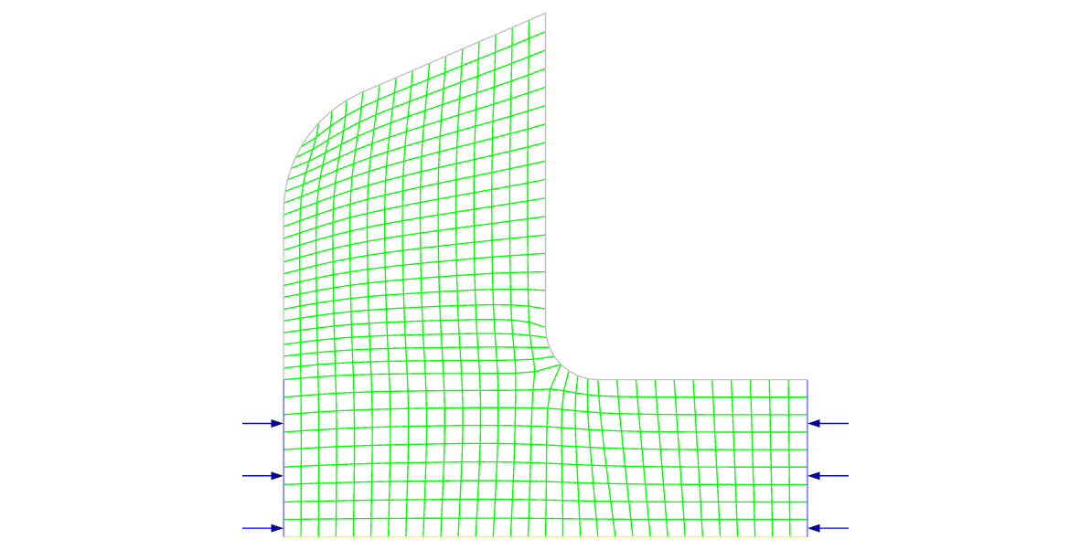
Display mesh#
graphics = Graphics(solver)
mesh = Mesh(solver, new_instance_name="mesh-1")
boundary_conditions = BoundaryConditions(solver)

graphics.picture.x_resolution = 650  # Horizontal resolution for clear visualization
graphics.picture.y_resolution = 450  # Vertical resolution matching typical aspect ratio

all_walls = mesh.surfaces_list.allowed_values()

mesh.surfaces_list = all_walls
mesh.options.edges = True
mesh.display()

graphics.views.auto_scale()
graphics.picture.save_picture(file_name="modeling_solidification_1.png")
Configure solver#
solver_general_settings = General(solver)

solver_general_settings.solver.two_dim_space = "swirl"

solver_general_settings.operating_conditions.gravity = {
    "enable": True,
    "components": [-9.81],
}
Enable models#
Note
Energy is auto-enabled with solidification
setup = Setup(solver)

setup.models.viscous.model = "laminar"

# Enable the Solidification/Melting
solver.tui.define.models.solidification_melting(
    "yes", "constant", "100000", "yes", "no"  # 100000 for the Mushy Zone Constant.
)
Define material#
materials = Materials(solver)

materials.database.copy_by_name(type="fluid", name="air", new_name="liquid-metal")

materials.fluid["liquid-metal"] = {
    "density": {
        "polynomial": {
            "coefficients": [
                8000,
                -0.1,
            ],  # [Density (kg/m³), Linear temp coefficient (kg/(m³·K))]
            "function_of": "temperature",
        },
        "option": "polynomial",
    },
    "viscosity": {"value": 0.00553},  # Pa·s
    "specific_heat": {"value": 680.0},  # J/kg·K
    "thermal_conductivity": {"value": 30.0},  # W/m·K
    "melting_heat": {"value": 100000.0},  # J/kg
    "tsolidus": {"value": 1150.0},  # K
    "tliqidus": {"value": 1150.0},  # K
}

# Assign material to fluid zone
setup.cell_zone_conditions.fluid["fluid"] = {"general": {"material": "liquid-metal"}}
Boundary conditions#
# Inlet: liquid injection
inlet = VelocityInlet(solver, name="inlet")

inlet.momentum.velocity_magnitude.value = 0.00101  # m/s
inlet.thermal.temperature.value = 1300  # K

# Outlet: solid pull-out (velocity inlet with axial + swirl)
outlet = VelocityInlet(solver, name="outlet")

outlet.momentum.velocity_specification_method = "Components"
outlet.momentum.swirl_angular_velocity = 1  # rad/s
outlet.momentum.velocity_components = [0.001, 0, 0]  # Axial = 0.001 m/s
outlet.thermal.temperature.value = 500  # K


conditions = BoundaryConditions(solver)

# Bottom wall: fixed temperature
conditions.wall["bottom-wall"] = {
    "thermal": {"thermal_condition": "Temperature", "temperature": 1300}  # K
}

# Free surface: Marangoni stress + convection
conditions.wall["free-surface"] = {
    "momentum": {
        "shear_condition": "Marangoni Stress",
        "surface_tension_gradient": -0.00036,  # N/m·K
    },
    "thermal": {
        "thermal_condition": "Convection",
        "free_stream_temp": 1500,  # K
        "heat_transfer_coeff": 100,  # W/m²·K
    },
}

# Side wall: fixed temperature
conditions.wall["side-wall"] = {
    "thermal": {"thermal_condition": "Temperature", "temperature": 1400}  # K
}

# Solid wall: rotating + cold
conditions.wall["solid-wall"] = {
    "momentum": {
        "wall_motion": "Moving Wall",
        "velocity_spec": "Rotational",
        "rotation_speed": 1,  # rad/s
    },
    "thermal": {"thermal_condition": "Temperature", "temperature": 500},  # K
}
Solution methods#
methods = Methods(solver)

methods.p_v_coupling.flow_scheme = "Coupled"
methods.spatial_discretization.discretization_scheme = {"pressure": "presto!"}
methods.pseudo_time_method.formulation = {"coupled_solver": "global-time-step"}
Disable flow equations#
controls = Controls(solver)

controls.equations = {"flow": False, "w-swirl": False}
Initialize flow field#
initialize = Initialization(solver)
initialize.hybrid_initialize()
Define custom field function#
results = Results(solver)

results.custom_field_functions.create(
    name="omegar", custom_field_function="1 * radial_coordinate"  # ω = 1 rad/s
)
Patch pull velocities#
# Axial pull velocity = 0.001 m/s
initialize.patch.calculate_patch(
    cell_zones=["fluid"],
    variable="x-pull-velocity",
    reference_frame="Relative to Cell Zone",
    use_custom_field_function=True,
    custom_field_function_name="omegar",
    value=0.001,
)

# Swirl pull velocity = ω × r
initialize.patch.calculate_patch(
    cell_zones=["fluid"],
    variable="z-pull-velocity",
    reference_frame="Relative to Cell Zone",
    use_custom_field_function=True,
    custom_field_function_name="omegar",
)
Pseudo-transient settings#
solver.settings.solution.run_calculation.pseudo_time_settings.time_step_method = {
    "time_step_method": "user-specified",
    "auto_time_size_calc_solid_zone": False,
}


calculation = RunCalculation(solver)
calculation.iterate(iter_count=20)
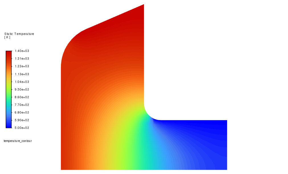
Post-processing#
temp_contour = Contour(solver, new_instance_name="temperature_contour")

temp_contour.coloring.option = "banded"
temp_contour.field = "temperature"
temp_contour.display()

graphics.views.restore_view(view_name="front")
graphics.views.auto_scale()
graphics.picture.save_picture(file_name="modeling_solidification_2.png")
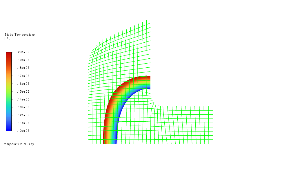
mushy_temp = Contour(solver, new_instance_name="temperature-mushy")
mushy_temp.coloring.option = "banded"
mushy_temp.field = "temperature"
mushy_temp.range_option = {
    "option": "auto-range-off",
    "auto_range_off": {"clip_to_range": True, "minimum": 1100, "maximum": 1200},
}
mushy_temp.display()

graphics.views.restore_view(view_name="front")
graphics.views.auto_scale()
graphics.picture.save_picture(file_name="modeling_solidification_3.png")
# Save steady state case
solver.settings.file.write_case_data(file_name="steady_state")
Enable transient flow and heat transfer#
solver_general_settings.solver.time = "unsteady-1st-order"  # First-order implicit

controls.equations = {"flow": True, "w-swirl": True}

controls.under_relaxation = {"delh": 0.1}
Transient controls#
solutions = Solution(solver)
solutions.run_calculation.transient_controls.time_step_count = 2
solutions.run_calculation.transient_controls.time_step_size = 0.1 # s
solutions.run_calculation.calculate()
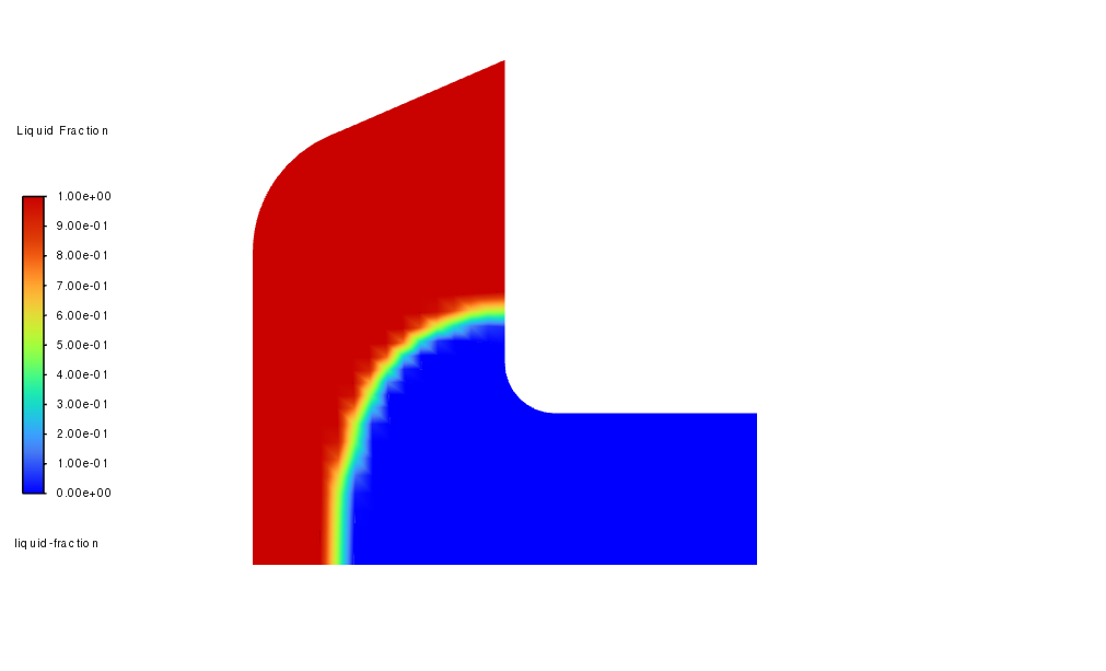
# Liquid fraction at t = 0.2 s
liquid_fraction_contour = Contour(solver, new_instance_name="liquid-fraction")
liquid_fraction_contour.field = "liquid-fraction"
liquid_fraction_contour.display()
graphics.views.auto_scale()
graphics.picture.save_picture(file_name="modeling_solidification_4.png")
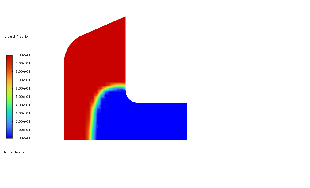
# Continue to t = 5.0 s (48 more steps)
solutions.run_calculation.transient_controls.time_step_count = 48

solutions.run_calculation.calculate()

# Liquid fraction at t = 5.0 s
liquid_fraction_contour_t_5_sec = Contour(solver, new_instance_name="liquid-fraction")

liquid_fraction_contour_t_5_sec.field = "liquid-fraction"
liquid_fraction_contour_t_5_sec.display()

graphics.views.auto_scale()
graphics.picture.save_picture(file_name="modeling_solidification_5.png")
# Save transient case
solver.settings.file.write_case_data(file_name="unsteady_state")
Close session#
solver.exit()
Summary#
In this example, we used PyFluent to model solidification in a Czochralski crystal growth process. The workflow begins with a steady conduction solution to establish the initial thermal field, followed by transient flow to capture natural and Marangoni-driven convection. Pull velocities are applied through a custom field function (ω × r), and surface tension gradients define Marangoni effects. This approach is efficient, fully scriptable, and easily adaptable to other casting or crystal growth simulations.
References:#
[1] Modeling Solidification, Ansys Fluent documentation.