Simulation of Steady Vortex in a Stirred Tank

Introduction

This tutorial demonstrates simulating vortex dynamics within continuous stirred tank reactors (CSTRs), which are extensively utilized in industries such as chemical, petrochemical, and pharmaceuticals for applications like fluid blending, crystallization, and pharmaceutical manufacturing. This tutorial includes step-by-step instructions on setting up the simulation using the MRF method, and employing best practices to accelerate free-surface flow simulations. Understanding vortex formation is crucial, as it often leads to undesirable effects like air entrainment and improper solid mixing. Identifying operating conditions that lead to vortex formation can help minimize these issues and ensure optimal liquid blending.

Problem Description

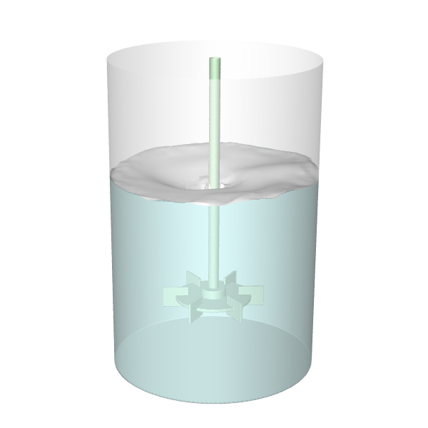
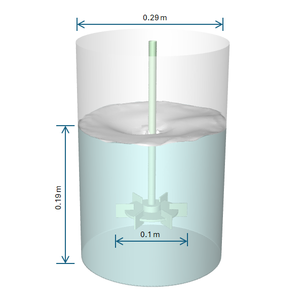
In this tutorial, we aim to model vortex formation in a stirred tank using a steady-state simulation. The setup involves an unbaffled cylindrical tank equipped with a Rushton turbine impeller, featuring the following specifications:

Tank Diameter : 0.29 meters Impeller Diameter: 0.1 meters Liquid Level: 0.19 meters Agitation Speed: 240 [rev min^-1]

The aim is to examine the vortex dynamics within the tank under given conditions.

Simulation Setup & Solution

Import required modules and classes

Import some direct settings classes which will be used in the following sections. These classes allow straightforward access to various settings without the need to navigate through the settings hierarchy.

import os

import imageio.v2 as imageio

import ansys.fluent.core as pyfluent
from ansys.fluent.core import Dimension, FluentMode, Precision
from ansys.fluent.core.examples import download_file
from ansys.fluent.core.solver import (  # noqa: E402
    LIC,
    CellRegister,
    CellZoneCondition,
    Contour,
    General,
    Graphics,
    Initialization,
    IsoClip,
    IsoSurface,
    Materials,
    Mesh,
    Methods,
    Models,
    NamedExpression,
    PlaneSurface,
    RunCalculation,
    Scene,
    WallBoundary,
)

Launch Fluent

Launch Fluent in 3D double precision solver mode.

solver_session = pyfluent.launch_fluent(
    mode=FluentMode.SOLVER,
    dimension=Dimension.THREE,
    precision=Precision.DOUBLE,
    cleanup_on_exit=True,
    cwd=os.getcwd(),
)
print(solver_session.get_fluent_version())  # Print the Fluent version
pyfluent.set_console_logging_level("INFO")  # Set the console logging level

Mesh

Download the mesh file and read it into the Fluent session.

vortex_mesh = download_file(
    "vortex-mixingtank.msh.h5",
    "pyfluent/examples/Steady-Vortex-VOF",
    save_path=os.getcwd(),
)

Define Constants

Define constants.

g = 9.81  # m/s^2

Read Mesh

Import the mesh file into the Fluent session.

solver_session.settings.file.read_case(file_name=vortex_mesh)

Display the mesh in Fluent and save the image to a file to examine locally.

# Create a middle plane to display the mesh
y_mid_plane = PlaneSurface(solver_session, new_instance_name="y_mid_plane")
y_mid_plane.method = "zx-plane"
y_mid_plane.y = 0
y_mid_plane.display()

# Define and display the mesh
mesh = Mesh(solver_session, new_instance_name="mesh")
mesh.surfaces_list = y_mid_plane.name()
mesh.options.edges = True
mesh.display()

# Create Graphics object to save the mesh image
graphics = Graphics(solver_session)
graphics.views.auto_scale()
if graphics.picture.use_window_resolution.is_active():
    graphics.picture.use_window_resolution = False

graphics.views.restore_view(view_name="top")
graphics.views.auto_scale()
graphics.picture.x_resolution = 600
graphics.picture.y_resolution = 600
graphics.picture.color_mode = "mono"
graphics.picture.save_picture(file_name="mesh.png")

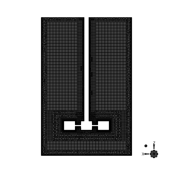
Polyhexcore Mesh for the Steady Vortex Simulation

Define General Settings

Set gravity

general_settings = General(solver_session)
general_settings.operating_conditions.gravity.enable = True
general_settings.operating_conditions.gravity.components = [0.0, 0.0, -g]

Copy Materials from Fluent Database

Copy water liquid materials from the Fluent database.

materials = Materials(solver_session)
materials.database.copy_by_name(type="fluid", name="water-liquid")

Define Named Expression for Agitation Speed

Create a named expression for the agitation speed and specify as an input parameter.

stirring_speed = NamedExpression(solver_session, new_instance_name="stirring_speed")

stirring_speed.definition = "240 [rev min^-1]"
stirring_speed.input_parameter = True

MRF zone parameters

Define MRF zone parameters for the mrf cell zone.

fluid_cell_zone = CellZoneCondition(solver_session, name="mrf")
fluid_cell_zone.reference_frame.frame_motion = True
fluid_cell_zone.reference_frame.reference_frame_axis_origin = [0, 0, 0]
fluid_cell_zone.reference_frame.reference_frame_axis_direction = [0, 0, 1]
fluid_cell_zone.reference_frame.mrf_omega.value = "stirring_speed"

Rotating Wall BC parameters

Define the rotating wall boundary condition for the shaft.

wall_boundary = WallBoundary(solver_session, name="shaft_tank")
wall_boundary.momentum.wall_motion = "Moving Wall"
wall_boundary.momentum.relative = False
wall_boundary.momentum.rotating = True
wall_boundary.momentum.rotation_axis_direction = [0, 0, 1]
wall_boundary.momentum.rotation_speed = "stirring_speed"

Physical Models: VOF

Enable the VOF multiphase model and update the curvature correction setting for the viscous model.

model_setup = Models(solver_session)
model_setup.multiphase.model = "vof"
model_setup.multiphase.vof_parameters.vof_formulation = "implicit"
model_setup.multiphase.vof_parameters.vof_cutoff = 1e-06
model_setup.multiphase.advanced_formulation.implicit_body_force = True

model_setup.viscous.options.curvature_correction = True

solution_methods = Methods(solver_session)
solution_methods.multiphase_numerics.solution_stabilization.execute_settings_optimization = (
    True
)
solution_methods.multiphase_numerics.solution_stabilization.execute_advanced_stabilization = (
    True
)

# Change phase names
solver_session.tui.define.phases.set_domain_properties.change_phases_names(
    "water", "air"
)
general_settings.solver.time = "steady"  # steady solver

Define Initial Conditions

Define initial conditions for the simulation and set up cell registers to define the initial liquid region in the tank and initialize the solution and set multipase numerics settings.

Note

Create a region of cells to patch the water volume fraction. Mark the cells from the bottom of the tank up to the specified height. Create a cell register named “liquid_patch”. Set Z-min to the tank’s minimum height coordinate and Z-max to 0.19 m. Utilize the minimum and maximum X & Y values to ensure cells across the entire tank diameter are included.

solution_initialization = Initialization(solver_session)
solution_initialization.reference_frame = "absolute"
solution_initialization.defaults["k"] = 0.001
solution_initialization.localized_turb_init.enabled = False

solver_session.settings.solution.cell_registers.create(name="liquid_patch")
cell_register = CellRegister(solver_session, name="liquid_patch")
cell_register.type = {
    "option": "hexahedron",
    "hexahedron": {
        "inside": True,
        "max_point": [100.0, 100.0, 0.19],
        "min_point": [-100.0, -100.0, -100.0],
    },
}

solution_initialization.initialize()

# Patch the water volume fraction in the defined cell register to set the initial
# liquid region in the tank.
# "mp" refers to the volume fraction of the primary phase (here water).
# Setting value=1 fills the patch region entirely with water.
solution_initialization.patch.calculate_patch(
    domain="water",
    cell_zones=[],
    registers=["liquid_patch"],
    variable="mp",
    reference_frame="Relative to Cell Zone",
    use_custom_field_function=False,
    value=1,
)

Postprocessing Setup

Define surfaces, meshes and scenes for postprocessing and visualization. e.g., to visualize the free surface and wetted walls and dry walls.

# Free surface iso-surface
solver_session.settings.results.surfaces.iso_surface.create(name="freesurface")
freesurface = IsoSurface(solver_session, name="freesurface")
freesurface.field = "water-vof"
freesurface.iso_values = [0.5]

# Wetted wall and dry wall iso-clips
solver_session.settings.results.surfaces.iso_clip.create(name="wet_wall")
wet_wall = IsoClip(solver_session, name="wet_wall")
wet_wall.field = "water-vof"
wet_wall.range = {
    "minimum": 0.5,
    "maximum": 1.0,
}
wet_wall.surfaces = ["wall_tank"]


solver_session.settings.results.surfaces.iso_clip.create(name="dry_wall")
dry_wall = IsoClip(solver_session, name="dry_wall")
dry_wall.field = "water-vof"
dry_wall.range = {
    "minimum": 0.0,
    "maximum": 0.499,
}
dry_wall.surfaces = ["wall_tank"]

# Meshes
internal_comp_mesh = Mesh(solver_session, new_instance_name="internals")
internal_comp_mesh.surfaces_list = [
    "wall_impeller",
    "shaft_mrf",
    "shaft_tank",
]
internal_comp_mesh.surfaces_list()

# dry wall
dry_wall_comp_mesh = Mesh(solver_session, new_instance_name="drywall")
dry_wall_comp_mesh.surfaces_list = ["dry_wall"]
dry_wall_comp_mesh.surfaces_list()

# wet wall
wet_wall_comp_mesh = Mesh(solver_session, new_instance_name="wetwall")
wet_wall_comp_mesh.surfaces_list = ["wet_wall"]
wet_wall_comp_mesh.surfaces_list()
wet_wall_comp_mesh.coloring.option = "manual"
wet_wall_comp_mesh.coloring.manual.faces = "pastel cyan"

# liquid level
liquidlevel_comp_mesh = Mesh(solver_session, new_instance_name="liquidlevel")
liquidlevel_comp_mesh.surfaces_list = ["freesurface"]
liquidlevel_comp_mesh.surfaces_list()
liquidlevel_comp_mesh.coloring.option = "manual"
liquidlevel_comp_mesh.coloring.manual.faces = "pastel cyan"


# Scenes
vortex_scene = Scene(solver_session, new_instance_name="scene-1")
vortex_scene.graphics_objects.add(name="liquidlevel")
vortex_scene.graphics_objects.add(name="drywall")
vortex_scene.graphics_objects.add(name="wetwall")
vortex_scene.graphics_objects.add(name="internals")

solver_session.settings.results.scene["scene-1"] = {
    "graphics_objects": {
        "liquidlevel": {
            "transparency": 50,
            "name": "tank",
            "colormap_position": 0,
            "colormap_left": 0.0,
            "colormap_bottom": 0.0,
            "colormap_width": 0.0,
            "colormap_height": 0.0,
        },
        "internals": {
            "transparency": 35,
            "name": "internals",
            "colormap_position": 0,
            "colormap_left": 0.0,
            "colormap_bottom": 0.0,
            "colormap_width": 0.0,
            "colormap_height": 0.0,
        },
        "drywall": {
            "transparency": 75,
            "name": "fs",
            "colormap_position": 0,
            "colormap_left": 0.0,
            "colormap_bottom": 0.0,
            "colormap_width": 0.0,
            "colormap_height": 0.0,
        },
        "wetwall": {
            "transparency": 75,
            "name": "wetwall",
            "colormap_position": 0,
            "colormap_left": 0.0,
            "colormap_bottom": 0.0,
            "colormap_width": 0.0,
            "colormap_height": 0.0,
        },
    }
}

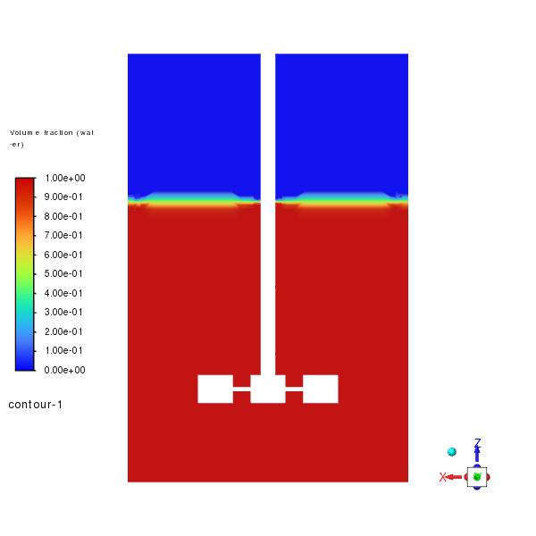
# Contour plot on Y-Mid plane
solver_session.settings.results.surfaces.iso_surface.create(name="ymid")
y_mid_iso_surface = IsoSurface(solver_session, name="ymid")
y_mid_iso_surface.field = "y-coordinate"
y_mid_iso_surface.iso_values = [0]

volume_fraction_contour = Contour(solver_session, new_instance_name="contour-1")
volume_fraction_contour.surfaces_list = y_mid_iso_surface.name()
volume_fraction_contour.field = "water-vof"
volume_fraction_contour.surfaces_list()
volume_fraction_contour.display()

graphics.views.restore_view(view_name="top")
graphics.views.auto_scale()
graphics.picture.color_mode = "color"
graphics.picture.use_window_resolution = False
graphics.picture.x_resolution = 600
graphics.picture.y_resolution = 600
graphics.picture.save_picture(file_name="contour.png")

Velocity Vectors

*The velocity vectors illustrate the flow patterns within the tank, highlighting the

complex interactions between the liquid and gas phases.*

# Animation Setup
solver_session.settings.solution.calculation_activity.solution_animations.create(
    "animation-2"
)
solver_session.settings.solution.calculation_activity.solution_animations[
    "animation-2"
] = {
    "animate_on": "scene-1",
    "frequency": 10,
    "storage_type": "png",
    "view": "top",
}

Save Initial Files & Run Calculation

Save the initial case file and run the calculation for 500 iterations.

solver_session.settings.file.write_case_data(file_name="vortex_init.cas.h5")

run_calculation = RunCalculation(solver_session)
run_calculation.iter_count = 50  # Iteration count keep it 50 for demo only purpose
run_calculation.calculate()

LIC Visualization

Set up the LIC (Line Integral Convolution) visualization for the midplane.

lic_visualization = LIC(solver_session, new_instance_name="lic-1")
lic_visualization.surfaces_list = y_mid_plane.name()
lic_visualization.field = "velocity-magnitude"
lic_visualization.lic_image_filter = "Strong Sharpen"
lic_visualization.lic_intensity_factor = 10
lic_visualization.texture_size = 10
lic_visualization.display()

graphics.views.restore_view(view_name="top")
graphics.views.auto_scale()
graphics.picture.use_window_resolution = False
graphics.picture.x_resolution = 600
graphics.picture.y_resolution = 600
graphics.picture.save_picture(file_name="lic-1.png")

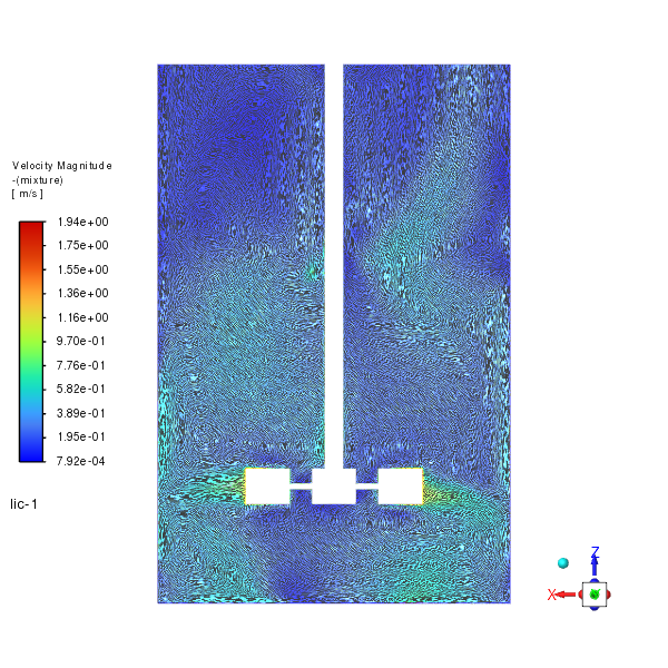
LIC Visualization

The LIC visualization provides a detailed view of the flow patterns within the tank.

Save Visualization of Final Vortex Shape & Write Simulation Files

Save the final vortex shape visualization and write the final case and data files.

vortex_scene.display()
graphics.views.restore_view(view_name="top")
graphics.views.auto_scale()

graphics.picture.use_window_resolution = False
graphics.picture.x_resolution = 600
graphics.picture.y_resolution = 600
graphics.picture.save_picture(file_name="vortex.png")

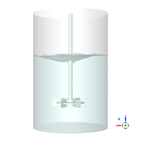
Vortex Shape Visualization

Steady vortex shape in the stirred tank.

# Save final case and data files
solver_session.settings.file.write_case_data(file_name="vortex_final.cas.h5")

Close Fluent

Exit the Fluent session.

solver_session.exit()

Generate GIF Animation: Vortex Formation

Create a GIF animation from the saved PNG images of the vortex formation using third-party library imageio.

Note

Install imageio package if not already installed. You can install it via pip: pip install imageio

png_dir = os.getcwd()
images = []
for file_name in sorted(os.listdir(png_dir)):
    if file_name.startswith("animation") and file_name.endswith(".png"):
        file_path = os.path.join(png_dir, file_name)
        images.append(imageio.imread(file_path))

imageio.mimsave(uri="vortex.gif", ims=images, duration=0.2)

Vortex Formation

The GIF animation illustrates the dynamic process of vortex formation within the stirred tank.