Note
Go to the end to download the full example code.
Single Battery Cell Using MSMD Battery Model Simulation#
Problem Description:#
Simulate a 14.6 Ah lithium-ion battery with a LiMn₂O₄ cathode and graphite anode using the Multi-Scale Multi-Domain (MSMD) battery model in Ansys Fluent. Evaluate the battery’s electrochemical and thermal performance under various discharge rates (e.g., 0.5C, 1C, 5C) and operating conditions, including normal operation, pulse discharge, and short-circuit scenarios. Key outputs include voltage, temperature, and state of charge.
Import modules#
import os

import ansys.fluent.core as pyfluent
from ansys.fluent.core import FluentMode, Precision, examples
Launch Fluent session#
Launch a Fluent solver session with required parameters
solver = pyfluent.launch_fluent(
    precision=Precision.DOUBLE, processor_count=4, mode=FluentMode.SOLVER
)
Download the mesh file#
Download the battery mesh file and save it to the current working directory.
unit_battery_mesh = examples.download_file(
    "unit_battery.msh.h5",
    "pyfluent/battery_thermal_simulation",
    save_path=os.getcwd(),
)
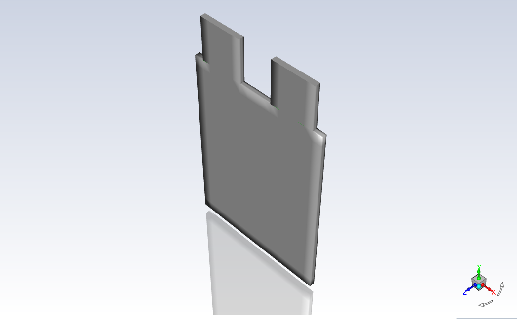
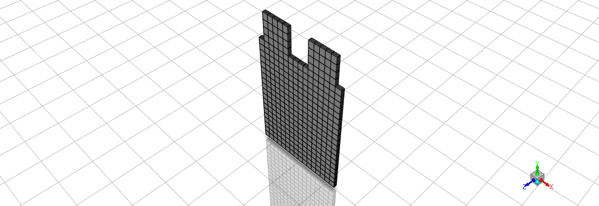
Read and display mesh#
Note
Graphics commands like restore_view and save_picture require GUI mode.
solver.settings.file.read_case(file_name=unit_battery_mesh)

# Get all the available wall boundary surfaces
all_walls = solver.settings.setup.boundary_conditions.wall.get_object_names()
mesh_object = solver.settings.results.graphics.mesh.create("mesh-1")
mesh_object.surfaces_list = all_walls
mesh_object.options.edges = True
mesh_object.display()

graphics_object = solver.settings.results.graphics
graphics_object.picture.x_resolution = 650
graphics_object.picture.y_resolution = 450
graphics_object.views.restore_view(view_name="isometric")
graphics_object.picture.save_picture(file_name="Single_Battery_Cell_Mesh.png")
Configure solver settings for battery model#
Use an unsteady first-order time solver for transient behavior.
solver.settings.setup.general.solver.time = "unsteady-1st-order"
Enable the battery model#
Activate the NTGK/DCIR model with a nominal cell capacity of 14.6 Ah. Enable Joule heat in passive zones and define zones and terminals. For a detailed guide on setting up a single battery cell,refer to the Reference [3].
battery = solver.settings.setup.models.battery
battery.enabled = True
battery.echem_model = "ntgk/dcir"
battery.zone_assignment.active_zone = ["e_zone"]
battery.zone_assignment.passive_zone = ["tab_nzone", "tab_pzone"]
battery.zone_assignment.negative_tab = ["tab_n"]
battery.zone_assignment.positive_tab = ["tab_p"]
Define materials for cell and tabs#
Note
Chemical formula values are arbitrary identifiers for demonstration.
Material definition for battery cell, positive tab and negative tab. User define
scalars are defined for e-material and positive material to specify the
electric conductivity with defined-per-uds and constant option respectively.
materials = [
    {
        "name": "e_material",
        "chemical_formula": "e",
        "density": 2092,
        "specific_heat": 678,
        "thermal_conductivity": 18.2,
        "uds_diffusivity": {
            "option": "defined-per-uds",
            "uds-0": 1190000,
            "uds-1": 983000,
        },
    },
    {
        "name": "p_material",
        "chemical_formula": "pmat",
        "density": 8978,
        "specific_heat": 381,
        "thermal_conductivity": 387.6,
        "uds_diffusivity": {"option": "constant", "value": 10000000},
    },
    {
        "name": "n_material",
        "chemical_formula": "nmat",
        "density": 8978,
        "specific_heat": 381,
        "thermal_conductivity": 387.6,
    },
]

solids = solver.settings.setup.materials.solid
for mat in materials:
    solids.create(mat["name"])
    solids[mat["name"]].chemical_formula = mat["chemical_formula"]
    solids[mat["name"]].density.value = mat["density"]
    solids[mat["name"]].specific_heat.value = mat["specific_heat"]
    solids[mat["name"]].thermal_conductivity.value = mat["thermal_conductivity"]
    if "uds_diffusivity" in mat:
        solids[mat["name"]].uds_diffusivity = {
            "option": mat["uds_diffusivity"]["option"]
        }
        if mat["uds_diffusivity"]["option"] == "defined-per-uds":
            solids[mat["name"]].uds_diffusivity.uds_diffusivities["uds-0"].value = mat[
                "uds_diffusivity"
            ]["uds-0"]
            solids[mat["name"]].uds_diffusivity.uds_diffusivities["uds-1"].value = mat[
                "uds_diffusivity"
            ]["uds-1"]
        else:
            solids[mat["name"]].uds_diffusivity.value = mat["uds_diffusivity"]["value"]
Assign materials to cell zones#
Map materials to respective zones.
cell_zones = [
    ("e_zone", "e_material"),
    ("tab_nzone", "n_material"),
    ("tab_pzone", "p_material"),
]

for zone, material in cell_zones:
    solver.settings.setup.cell_zone_conditions.solid[zone].general.material = material
Define boundary conditions#
Set convective heat transfer on external surfaces.
wall = solver.settings.setup.boundary_conditions.wall
wall["wall_active"].thermal.thermal_condition = "Convection"
wall["wall_active"].thermal.heat_transfer_coeff.value = 5

# API to copy similar boundary condition
solver.settings.setup.boundary_conditions.copy(
    from_="wall_active", to=["wall_n", "wall_p"]
)
Configure solution settings#
Disable flow and turbulence equations, since residual criteria are set to none
solver.settings.solution.controls.equations["flow"] = False
solver.settings.solution.controls.equations["kw"] = False

solver.settings.solution.monitor.residual.options.criterion_type = "none"
Create report definitions#
Monitor average voltage and maximum temperature.
avg_surface_voltage_report_def = (
    solver.settings.solution.report_definitions.surface.create("surface_voltage")
)
avg_surface_voltage_report_def.report_type = "surface-areaavg"
avg_surface_voltage_report_def.field = "passive-zone-potential"
avg_surface_voltage_report_def.surface_names = ["tab_p"]

max_temp_report_def = solver.settings.solution.report_definitions.volume.create(
    "max_temperature"
)
max_temp_report_def.report_type = "volume-max"
max_temp_report_def.field = "temperature"
max_temp_report_def.cell_zones = ["e_zone", "tab_nzone", "tab_pzone"]

surf_voltage_report_files = solver.settings.solution.monitor.report_files.create(
    "surface_voltage_file"
)
surf_voltage_report_files.report_defs = ["flow-time", "surface_voltage"]
surf_voltage_report_files.file_name = "ntgk-1c.out"
surf_voltage_report_files.print = True

max_temp_report_file = solver.settings.solution.monitor.report_files.create(
    "max_temperature_file"
)
max_temp_report_file.report_defs = ["max_temperature"]
max_temp_report_file.file_name = "max-temp-1c.out"
max_temp_report_file.print = True

report_plots = solver.settings.solution.monitor.report_plots

voltage_plot = report_plots.create("surface_voltage_plot")
voltage_plot.report_defs = ["surface_voltage"]
voltage_plot.print = True
voltage_plot.axes.x.number_format.precision = 0
voltage_plot.axes.y.number_format.precision = 2

temp_plot = report_plots.create("max_temperature_plot")
temp_plot.report_defs = ["max_temperature"]
temp_plot.print = True
temp_plot.axes.x.number_format.precision = 0
temp_plot.axes.y.number_format.precision = 2
Run the simulation#
solver.settings.solution.initialization.standard_initialize()
transient_controls = solver.settings.solution.run_calculation.transient_controls
transient_controls.time_step_size = 30
transient_controls.time_step_count = 100
solver.settings.solution.run_calculation.calculate()
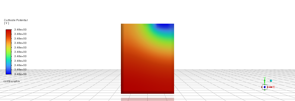
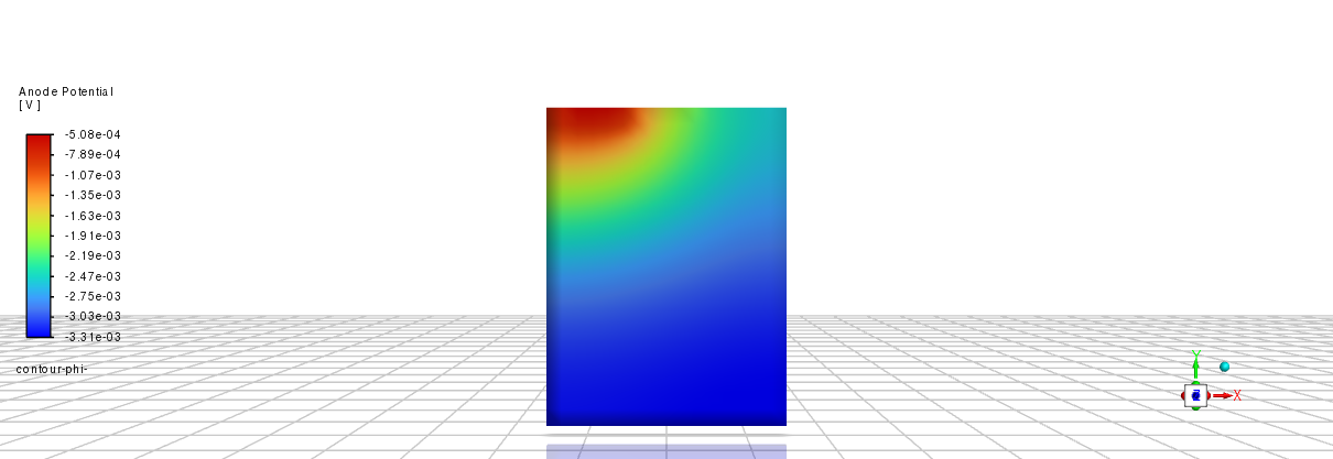
Post-process results#
Generate contour and vector plots.
contours = solver.settings.results.graphics.contour
contour_list = [
{
"name": "contour-phi+",
"field": "cathode-potential",
"surfaces": ["wall_active"],
"file_name": "Single_Battery_Cell_1.png",
},
{
"name": "contour-phi-",
"field": "anode-potential",
"surfaces": ["wall_active"],
"file_name": "Single_Battery_Cell_2.png",
},
{
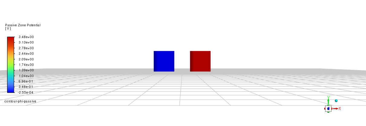
"name": "contour-phi-passive",
"field": "passive-zone-potential",
"surfaces": ["tab_n", "tab_p", "wall_n", "wall_p"],
"file_name": "Single_Battery_Cell_3.png",
},
{
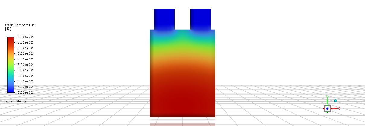
"name": "contour-temp",
"field": "temperature",
"surfaces": ["wall_p", "wall_active", "tab_p", "tab_n", "wall_n"],
"file_name": "Single_Battery_Cell_4.png",
},
]
# Create, display, and save contour plots
for contour in contour_list:
# Create the contour
contours.create(contour["name"])
current = contours[contour["name"]]
current.field = contour["field"]
current.surfaces_list = contour["surfaces"]
current.range_options.compute()
# Set the view
graphics_object.views.restore_view(view_name="front")
# display the current contour
current.display()
# Save the contour plot as an image
graphics_object.picture.save_picture(file_name=contour["file_name"])
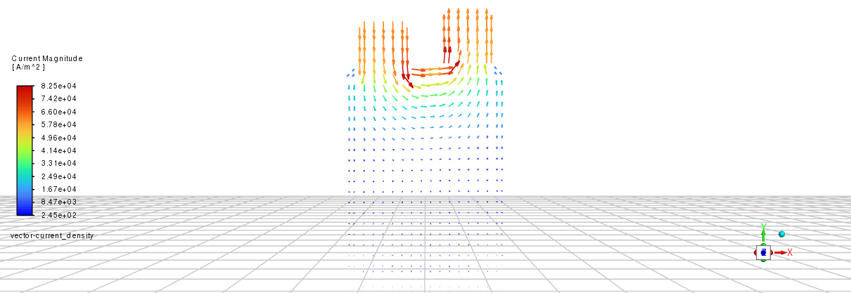
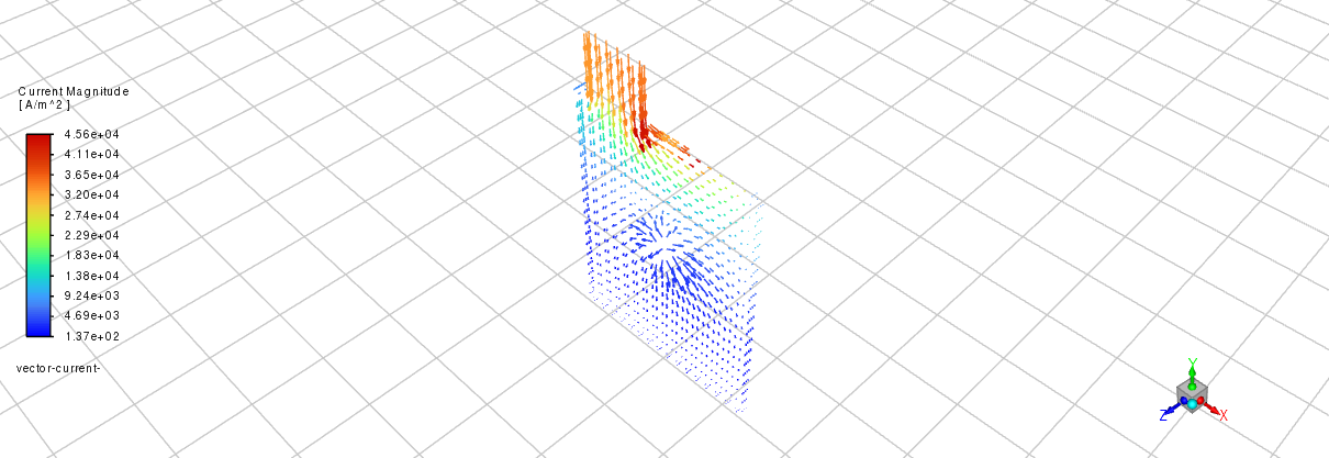
# Create and configure vector plot
vector_plot = solver.settings.results.graphics.vector.create("vector-current_density")
vector_plot.vector_field = "current-density-j"
vector_plot.field = "current-magnitude"
vector_plot.surfaces_list = ["wall_n", "wall_p", "wall_active", "tab_n", "tab_p"]
vector_plot.options.vector_style = "arrow"
vector_plot.range_options.compute()
# Set view, display, and save the vector plot image
graphics_object.views.restore_view(view_name="front")
vector_plot.display()
graphics_object.picture.save_picture(file_name="Single_Battery_Cell_5.png")
# Save case file for ROM simulation
solver.settings.file.write_case(file_name="unit_battery.cas.h5")
# Save case and data for short circuit simulation
solver.settings.file.write_case_data(file_name="ntgk") # Save case data
Run simulations at different C-rates#
Simulate at 0.5C and 5C discharge rates with adjusted time steps.
solver.settings.setup.models.battery.eload_condition.eload_settings.crate_value = 0.5

# Get report files
report_files = solver.settings.solution.monitor.report_files

# Update report file names for 0.5 c rate simulation for existing report files
report_files["surface_voltage_file"].file_name = "ntgk-0.5c.out"
report_files["max_temperature_file"].file_name = "max-temp-0.5c.out"
solver.settings.solution.initialization.standard_initialize()
solver.settings.solution.run_calculation.transient_controls.time_step_count = 230
solver.settings.solution.run_calculation.calculate()

solver.settings.setup.models.battery.eload_condition.eload_settings.crate_value = 5

# Update report file names for 5 c rate simulation for existing report files
report_files["surface_voltage_file"].file_name = "ntgk-5c.out"
report_files["max_temperature_file"].file_name = "max-temp-5c.out"
solver.settings.solution.initialization.standard_initialize()
solver.settings.solution.run_calculation.transient_controls.time_step_count = 23
solver.settings.solution.run_calculation.calculate()
Reduced Order Method (ROM) setup#
Apply ROM for computational efficiency.
solver.settings.file.read_case(file_name="unit_battery.cas.h5")
solver.settings.solution.initialization.standard_initialize()
solver.settings.solution.run_calculation.transient_controls.time_step_size = 30
solver.settings.solution.run_calculation.transient_controls.time_step_count = 3
solver.settings.solution.run_calculation.calculate()
solver.settings.setup.models.battery.solution_method = "msmd-rom"
solver.settings.setup.models.battery.solution_option.option_settings.number_substeps = (
10
)
solver.settings.solution.run_calculation.transient_controls.time_step_size = 30
solver.settings.solution.run_calculation.transient_controls.time_step_count = 100
solver.settings.solution.run_calculation.calculate()
# Generate contour and vector plots for ROM results.
contours = solver.settings.results.graphics.contour
contour_list = [
{
"name": "contour_cathode_potential",
"field": "cathode-potential",
"surfaces": ["wall_active"],
},
{
"name": "contour_anode_potential",
"field": "anode-potential",
"surfaces": ["wall_active"],
},
{
"name": "contour_passive_potential",
"field": "passive-zone-potential",
"surfaces": ["tab_n", "tab_p", "wall_n", "wall_p"],
},
{
"name": "contour_temperature",
"field": "temperature",
"surfaces": ["wall_p", "wall_active", "tab_p", "tab_n", "wall_n"],
},
]
for contour in contour_list:
contours.create(contour["name"])
contours[contour["name"]].field = contour["field"]
contours[contour["name"]].surfaces_list = contour["surfaces"]
contours[contour["name"]].range_options.compute()
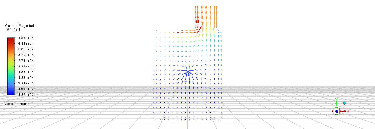
vectors = solver.settings.results.graphics.vector.create("vector-current_density")
vectors.vector_field = "current-density-j"
vectors.field = "current-magnitude"
vectors.surfaces_list = [
"wall_n",
"wall_p",
"wall_active",
"tab_n",
"tab_p",
]
vectors.options.vector_style = "arrow"
vectors.range_options.compute()
# Set view, display, and save the vector plot image
graphics_object.views.restore_view(view_name="front")
vectors.display()
graphics_object.picture.save_picture(file_name="Single_Battery_Cell_6.png")
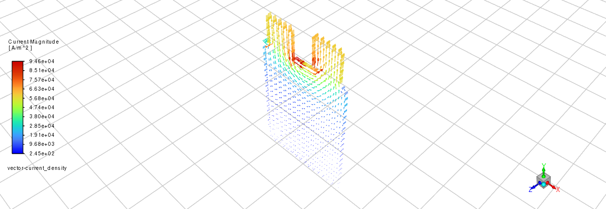
Vector current density for ROM model (faster with identical results).
Simulate short-circuit#
Apply low external resistance and define a short-circuit region.
solver.settings.file.read_case(file_name="ntgk.cas.h5")

solver.settings.setup.models.battery.eload_condition.eload_settings.eload_type = (
    "specified-resistance"
)
solver.settings.setup.models.battery.eload_condition.eload_settings.external_resistance = (
    0.5
)

# Create a new cell register named "register_patch"
patch = solver.settings.solution.cell_registers.create(name="register_patch")
patch.type.option = "hexahedron"

# Configure the hexahedron box
patch.type.hexahedron.inside = True
patch.type.hexahedron.min_point = [-0.01, -0.01, -1.0]
patch.type.hexahedron.max_point = [0.01, 0.02, 1.0]

solver.settings.solution.initialization.standard_initialize()

# Patch initialization
solver.settings.solution.initialization.patch.calculate_patch(
    domain="",
    cell_zones=[],
    registers=["register_patch"],
    variable="battery-short-resistance",
    reference_frame="Relative to Cell Zone",
    use_custom_field_function=False,
    custom_field_function_name="",
    value=5e-07,
)

solver.settings.solution.run_calculation.transient_controls.time_step_size = 1
solver.settings.solution.run_calculation.transient_controls.time_step_count = 5
solver.settings.solution.run_calculation.calculate()

solver.settings.file.write_case_data(file_name="ntgk_short_circuit.cas.h5")

solver.settings.results.report.surface_integrals.area_weighted_avg(
    report_of="passive-zone-potential", surface_names=["tab_p"], write_to_file=False
)
solver.settings.results.report.volume_integrals.volume_integral(
    cell_function="total-current-source", cell_zones=["e_zone"], write_to_file=False
)

vector = solver.settings.results.graphics.vector
vector_negative = vector.create("vector_negative_current")
vector_negative.vector_field = "current-density-jn"
vector_negative.field = "current-magnitude"
vector_negative.surfaces_list = [
    "wall_n",
    "wall_p",
    "wall_active",
]
vector_negative.options.vector_style = "arrow"
vector_negative.range_options.compute()
graphics_object.views.restore_view(view_name="front")
vector_negative.display()
graphics_object.picture.save_picture(file_name="Single_Battery_Cell_9.png")
Negative current vector plot after short circuit.
vector_positive = vector.create("vector_positive_current")
vector_positive.vector_field = "current-density-jp"
vector_positive.field = "current-magnitude"
vector_positive.surfaces_list = [
    "wall_n",
    "wall_p",
    "wall_active",
]
vector_positive.options.vector_style = "arrow"
vector_positive.range_options.compute()

graphics_object.views.restore_view(view_name="front")
vector_positive.display()
graphics_object.picture.save_picture(file_name="Single_Battery_Cell_10.png")
Positive current vector plot after short circuit.
temp_contour = solver.settings.results.graphics.contour.create("temperature-contour")
temp_contour.field = "temperature"
temp_contour.surfaces_list = all_walls
temp_contour.range_options.compute()

graphics_object.views.restore_view(view_name="front")
temp_contour.display()
graphics_object.picture.save_picture(file_name="Single_Battery_Cell_11.png")
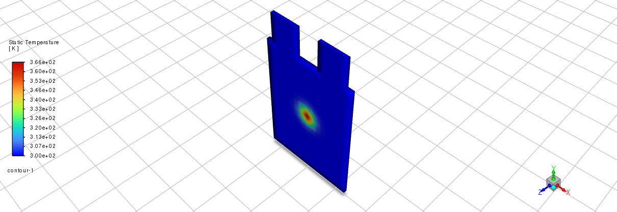
Temperature contour plot after short circuit.
Close the solver#
solver.exit()
References:#
[1] U. S. Kim et al, “Effect of electrode configuration on the thermal behavior of a lithium-polymer battery”, Journal of Power Sources, Volume 180 (2), pages 909-916, 2008.
[2] U. S. Kim, et al., “Modeling the Dependence of the Discharge Behavior of a Lithium-Ion Battery on the Environmental Temperature”, J. of Electrochemical Soc., Volume 158 (5), pages A611-A618, 2011.
[3] Simulating a Single Battery Cell Using the MSMD Battery Model, Ansys Fluent documentation.