Modeling Cavitation

This example examines the pressure-driven cavitating flow of water through a sharp-edged orifice. This is a typical configuration in fuel injectors, and brings a challenge to the physics and numerics of cavitation models because of the high pressure differentials involved and the high ratio of liquid to vapor density.

This example uses the multiphase modeling capability of Ansys Fluent, and will be able to predict the strong cavitation near the orifice after flow separation at a sharp edge.

Workflow tasks

This example demonstrates how to do the following:

• Set boundary conditions for internal flow

• Use the mixture model with cavitation effects

• Calculate a solution using the pressure-based coupled solver

Problem description

The problem considers the cavitation caused by the flow separation after a sharp-edged orifice. The flow is pressure driven, with an inlet pressure of 500 kPa and an outlet pressure of 95 kPa. The orifice diameter is 4 mm, and the geometrical parameters of the orifice are D/d = 2.88 and L/d = 4, where D, d, and L are the inlet diameter, orifice diameter, and orifice length respectively.

Example Setup

Before you can begin, you must set up the example and initialize this workflow.

Launch Fluent

Perform required imports, which includes downloading and importing the geometry file.

import ansys.fluent.core as pyfluent
from ansys.fluent.core import examples

cav_file = examples.download_file("cav.msh.gz", "pyfluent/cavitation")

Download successful. File path:
/home/ansys/.local/share/ansys_fluent_core/examples/cav.msh.gz

Launch a Fluent session in the 2d solution mode with double precision running on four processors.

solver = pyfluent.launch_fluent(
    precision="double",
    processor_count=4,
    mode="solver",
    version="2d",
)

Read the mesh that was downloaded.

solver.file.read_mesh(file_name=cav_file)

solver.mesh.check()

Specify an axisymmetric model.

solver.setup.general.solver.two_dim_space = "axisymmetric"

Enable the multiphase mixture model.

solver.setup.models.multiphase.models = "mixture"

solver.tui.define.models.multiphase.mixture_parameters("no", "implicit")

Enable the k-ω SST turbulence model.

solver.setup.models.viscous = {
    "model": "k-omega",
    "k_omega_model": "sst",
}

Define materials

Create a material named water, using 1000 kg/m3 for density and 0.001 kg/m–s for viscosity. Then, copy water vapor properties from the database and modify the copy by changing the density to 0.02558 kg/m3 and the viscosity to 1.26e-06 kg/m–s.

solver.setup.materials.fluid["water"] = {
    "density": {
        "option": "constant",
        "value": 1000,
    },
    "viscosity": {
        "option": "constant",
        "value": 0.001,
    },
}

solver.setup.materials.database.copy_by_name(type="fluid", name="water-vapor")

solver.setup.materials.fluid["water-vapor"] = {
    "density": {"value": 0.02558},
    "viscosity": {"value": 1.26e-06},
}

Phases

Change the name of the primary phase to “liquid” and the secondary phase to “water-vapor”. Then, enable the cavitation model and set the number of mass transfer mechanisms to 1. Finally, specify cavitation as a mass transfer mechanism occurring from the liquid to the vapor.

solver.tui.define.phases.set_domain_properties.change_phases_names("vapor", "liquid")

solver.tui.define.phases.set_domain_properties.phase_domains.liquid.material(
    "yes", "water"
)

solver.tui.define.phases.set_domain_properties.phase_domains.vapor.material(
    "yes", "water-vapor"
)

solver.tui.define.phases.set_domain_properties.interaction_domain.heat_mass_reactions.mass_transfer(
    1, "liquid", "vapor", "cavitation", "1", "no", "no", "no"
)

Boundary Conditions

For the first inlet momentum boundary conditions set the direction specification method to ‘normal to boundary’, gauge total pressure as 500 kPa and supersonic or initial gauge pressure as 449 kPa.

For the turbulence settings choose ‘Intensity and Viscosity Ratio’ for turbulent specification. Set turbulent intensity and turbulent viscosity ratio to 0.05 and 10 respectively.

inlet_1 = solver.setup.boundary_conditions.pressure_inlet["inlet_1"].phase

inlet_1["mixture"] = {
    "momentum": {
        "gauge_total_pressure": {"value": 500000},
        "supersonic_or_initial_gauge_pressure": {"value": 449000},
        "direction_specification_method": "Normal to Boundary",
    },
    "turbulence": {
        "turbulent_specification": "Intensity and Viscosity Ratio",
        "turbulent_intensity": 0.05,
        "turbulent_viscosity_ratio_real": 10,
    },
}

Before copying inlet_1’s boundary conditions to inlet_2, set the vapor fraction to 0.

inlet_1["vapor"] = {
    "multiphase": {
        "volume_fraction": {"value": 0},
    },
}

solver.setup.boundary_conditions.copy(from_="inlet_1", to="inlet_2")

For the outlet boundary conditions, set the gauge pressure as 95 kPa. Use the same turbulence and volume fraction settings as the inlets.

outlet = solver.setup.boundary_conditions.pressure_outlet["outlet"].phase

outlet["mixture"] = {
    "momentum": {
        "gauge_pressure": {"value": 95000},
    },
    "turbulence": {
        "turbulent_specification": "Intensity and Viscosity Ratio",
        "turbulent_intensity": 0.04,
        "turbulent_viscosity_ratio_real": 10,
    },
}

outlet["vapor"] = {
    "multiphase": {
        "volume_fraction": {"value": 0},
    },
}

Operating Conditions

Set the operating pressure to 0.

solver.setup.general.operating_conditions.operating_pressure = 0

Solution

To configure the discretization scheme, set ‘first order upwind’ method for turbulent kinetic energy and turbulent dissipation rate, ‘quick’ for the momentum and volume fraction, and ‘presto!’ for pressure.

methods = solver.solution.methods

methods.discretization_scheme = {
    "k": "first-order-upwind",
    "mom": "quick",
    "mp": "quick",
    "omega": "first-order-upwind",
    "pressure": "presto!",
}

For the pressure velocity coupling scheme choose ‘Coupled’. Set the pseudo time step method to ‘global time step’ and enable ‘High Order Term Relaxation’. Then, set the explicit relaxation factor for ‘Volume Fraction’ to 0.3.

methods.p_v_coupling.flow_scheme = "Coupled"

methods.pseudo_time_method.formulation.coupled_solver = "global-time-step"

methods.high_order_term_relaxation.enable = True

solver.solution.controls.pseudo_time_explicit_relaxation_factor.global_dt_pseudo_relax[
    "mp"
] = 0.3

To plot the residuals, enable plotting and set the convergence criteria to 1e-05 for x-velocity, y-velocity, k, omega, and vf-vapor. Enable the specified initial pressure then initialize the solution with hybrid initialization.

solver.solution.monitor.residual.options.plot = True

resid_eqns = solver.solution.monitor.residual.equations

resid_eqns["continuity"].absolute_criteria = 1e-5
resid_eqns["x-velocity"].absolute_criteria = 1e-5
resid_eqns["y-velocity"].absolute_criteria = 1e-5
resid_eqns["k"].absolute_criteria = 1e-5
resid_eqns["omega"].absolute_criteria = 1e-5
resid_eqns["vf-vapor"].absolute_criteria = 1e-5

initialization = solver.solution.initialization

initialization.initialization_type = "hybrid"
initialization.hybrid_init_options.general_settings.initial_pressure = True
initialization.hybrid_initialize()

Save and Run

Save the case file ‘cav.cas.h5’. Then, start the calculation by requesting 500 iterations. Save the final case file and the data.

solver.file.write_case(file_name="cav")

solver.solution.run_calculation.iterate(iter_count=500)

solver.file.write_case_data(file_name="cav")

Post Processing

Since Fluent is being run without the GUI, we will need to export plots as picture files. Edit the picture settings to use a custom resolution so that the images are large enough.

graphics = solver.results.graphics
# use_window_resolution option not available inside containers
if not solver.connection_properties.inside_container:
    graphics.picture.use_window_resolution = False
graphics.picture.x_resolution = 1920
graphics.picture.y_resolution = 1440

Create contour plots

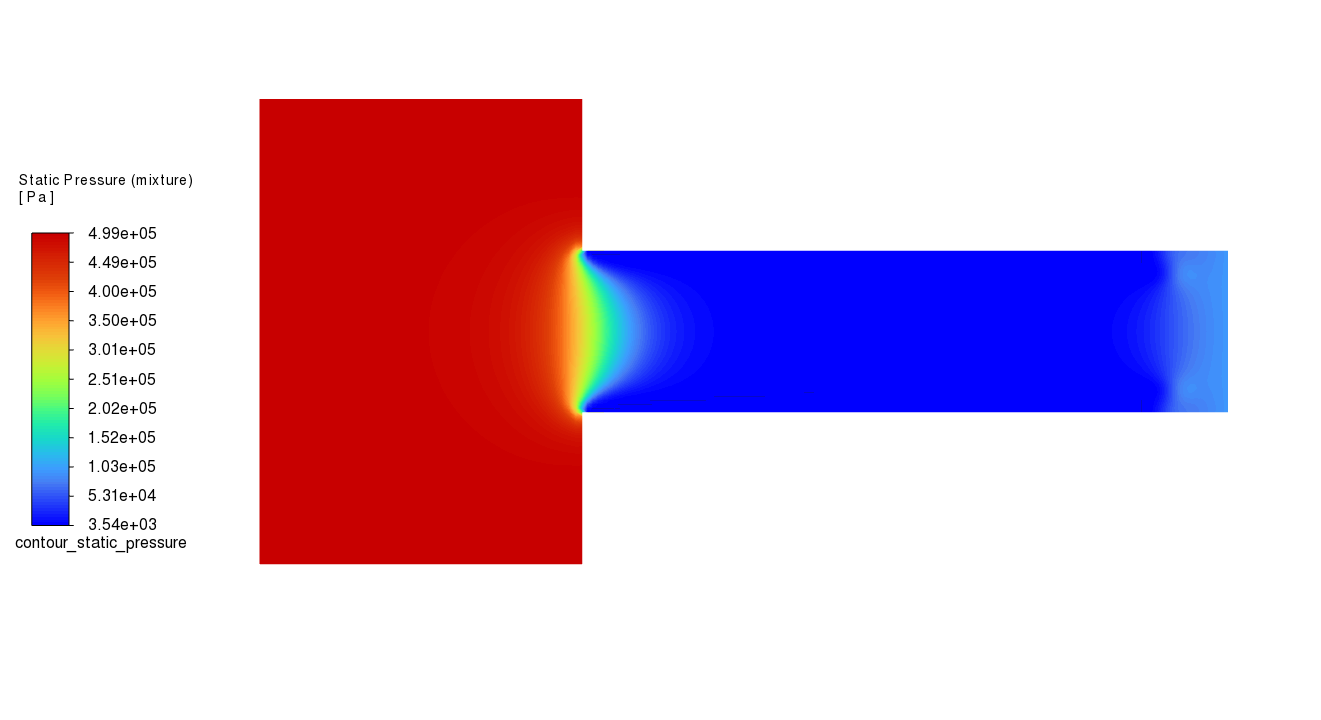
Create a contour plot for static pressure, turbulent kinetic energy and the volume fraction of water vapor. For each plot enable banded coloring and filled option.

graphics = solver.results.graphics

graphics.contour["contour_static_pressure"] = {
    "coloring": {
        "option": "banded",
        "smooth": False,
    },
    "field": "pressure",
    "filled": True,
}

Mirror the display around the symmetry plane to show the full model.

solver.tui.display.set.mirror_zones(["symm_2", "symm_1"])

graphics.contour["contour_static_pressure"].display()

graphics.picture.save_picture(file_name="contour_static_pressure.png")

graphics.contour.create("contour_tke")

graphics.contour["contour_tke"] = {
    "coloring": {
        "option": "banded",
        "smooth": False,
    },
    "field": "turb-kinetic-energy",
    "filled": True,
}

graphics.contour["contour_tke"].display()

graphics.picture.save_picture(file_name="contour_tke.png")

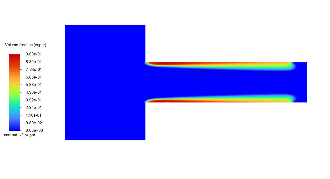
graphics.contour.create("contour_vf_vapor")

graphics.contour["contour_vf_vapor"] = {
    "coloring": {
        "option": "banded",
        "smooth": False,
    },
    "field": "vapor-vof",
    "filled": True,
}

graphics.contour["contour_vf_vapor"].display()

graphics.picture.save_picture(file_name="contour_vf_vapor.png")

# Save case to 'cav.cas.h5' and exit

solver.file.write_case(file_name="cav")

solver.exit()