Note
Go to the end to download the full example code.
Fluent setup and solution using settings objects#
This example sets up and solves a three-dimensional turbulent fluid flow and heat transfer problem in a mixing elbow, which is common in piping systems in power plants and process industries. Predicting the flow field and temperature field in the area of the mixing region is important to designing the junction properly.
This example uses settings objects.
Problem description
A cold fluid at 20 deg C flows into the pipe through a large inlet. It then mixes
with a warmer fluid at 40 deg C that enters through a smaller inlet located at
the elbow. The pipe dimensions are in inches, and the fluid properties and
boundary conditions are given in SI units. Because the Reynolds number for the
flow at the larger inlet is 50, 800, a turbulent flow model is required.
Perform required imports#
Perform required imports, which includes downloading and importing the geometry file.
import os

import ansys.fluent.core as pyfluent
from ansys.fluent.core import examples

import_file_name = examples.download_file(
    "mixing_elbow.msh.h5",
    "pyfluent/mixing_elbow",
    save_path=os.getcwd(),
)
Launch Fluent#
Launch Fluent as a service in solver mode with double precision running on two processors and print Fluent version.
solver_session = pyfluent.launch_fluent(
    precision="double",
    processor_count=2,
    mode="solver",
)
print(solver_session.get_fluent_version())
Import mesh and perform mesh check#
Import the mesh and perform a mesh check, which lists the minimum and maximum x, y, and z values from the mesh in the default SI units of meters. The mesh check also reports a number of other mesh features that are checked. Any errors in the mesh are reported. Ensure that the minimum volume is not negative because Fluent cannot begin a calculation when this is the case.
solver_session.settings.file.read_case(file_name=import_file_name)
solver_session.settings.mesh.check()
Enable heat transfer#
Enable heat transfer by activating the energy equation.
solver_session.settings.setup.models.energy.enabled = True
Create material#
Create a material named "water-liquid".
solver_session.settings.setup.materials.database.copy_by_name(
    type="fluid", name="water-liquid"
)
Set up cell zone conditions#
Set up the cell zone conditions for the fluid zone (elbow-fluid). Set material
to "water-liquid".
solver_session.settings.setup.cell_zone_conditions.fluid[
    "elbow-fluid"
].general.material = "water-liquid"
Set up boundary conditions for CFD analysis#
Set up the boundary conditions for the inlets, outlet, and walls for CFD analysis.
# cold inlet (cold-inlet), Setting: Value:
# Velocity Specification Method: Magnitude, Normal to Boundary
# Velocity Magnitude: 0.4 [m/s]
# Specification Method: Intensity and Hydraulic Diameter
# Turbulent Intensity: 5 [%]
# Hydraulic Diameter: 4 [inch]
# Temperature: 293.15 [K]
cold_inlet = solver_session.settings.setup.boundary_conditions.velocity_inlet[
    "cold-inlet"
]

cold_inlet.momentum.velocity_magnitude.value = 0.4
cold_inlet.turbulence.turbulence_specification = "Intensity and Hydraulic Diameter"
cold_inlet.turbulence.turbulent_intensity = 0.05
cold_inlet.turbulence.hydraulic_diameter = "4 [in]"
cold_inlet.thermal.temperature.value = 293.15

# hot inlet (hot-inlet), Setting: Value:
# Velocity Specification Method: Magnitude, Normal to Boundary
# Velocity Magnitude: 1.2 [m/s]
# Specification Method: Intensity and Hydraulic Diameter
# Turbulent Intensity: 5 [%]
# Hydraulic Diameter: 1 [inch]
# Temperature: 313.15 [K]
hot_inlet = solver_session.settings.setup.boundary_conditions.velocity_inlet[
    "hot-inlet"
]

hot_inlet.momentum.velocity_magnitude.value = 1.2
hot_inlet.turbulence.turbulence_specification = "Intensity and Hydraulic Diameter"
hot_inlet.turbulence.hydraulic_diameter = "1 [in]"
hot_inlet.thermal.temperature.value = 313.15

# pressure outlet (outlet), Setting: Value:
# Backflow Turbulent Intensity: 5 [%]
# Backflow Turbulent Viscosity Ratio: 4

solver_session.settings.setup.boundary_conditions.pressure_outlet[
    "outlet"
].turbulence.turbulent_viscosity_ratio = 4
solver_session.settings.setup.boundary_conditions.pressure_outlet[
    "outlet"
].turbulence.backflow_turbulent_intensity = 0.05
Initialize flow field#
Initialize the flow field using hybrid initialization.
solver_session.settings.solution.initialization.hybrid_initialize()
Solve for 150 iterations#
Solve for 150 iterations.
solver_session.settings.solution.run_calculation.iterate(iter_count=150)
Configure graphics picture export#
Since Fluent is being run without the GUI, we will need to export plots as picture files. Edit the picture settings to use a custom resolution so that the images are large enough.
graphics = solver_session.settings.results.graphics
# use_window_resolution option not active inside containers or Ansys Lab environment
if graphics.picture.use_window_resolution.is_active():
    graphics.picture.use_window_resolution = False

graphics.picture.x_resolution = 1920
graphics.picture.y_resolution = 1440
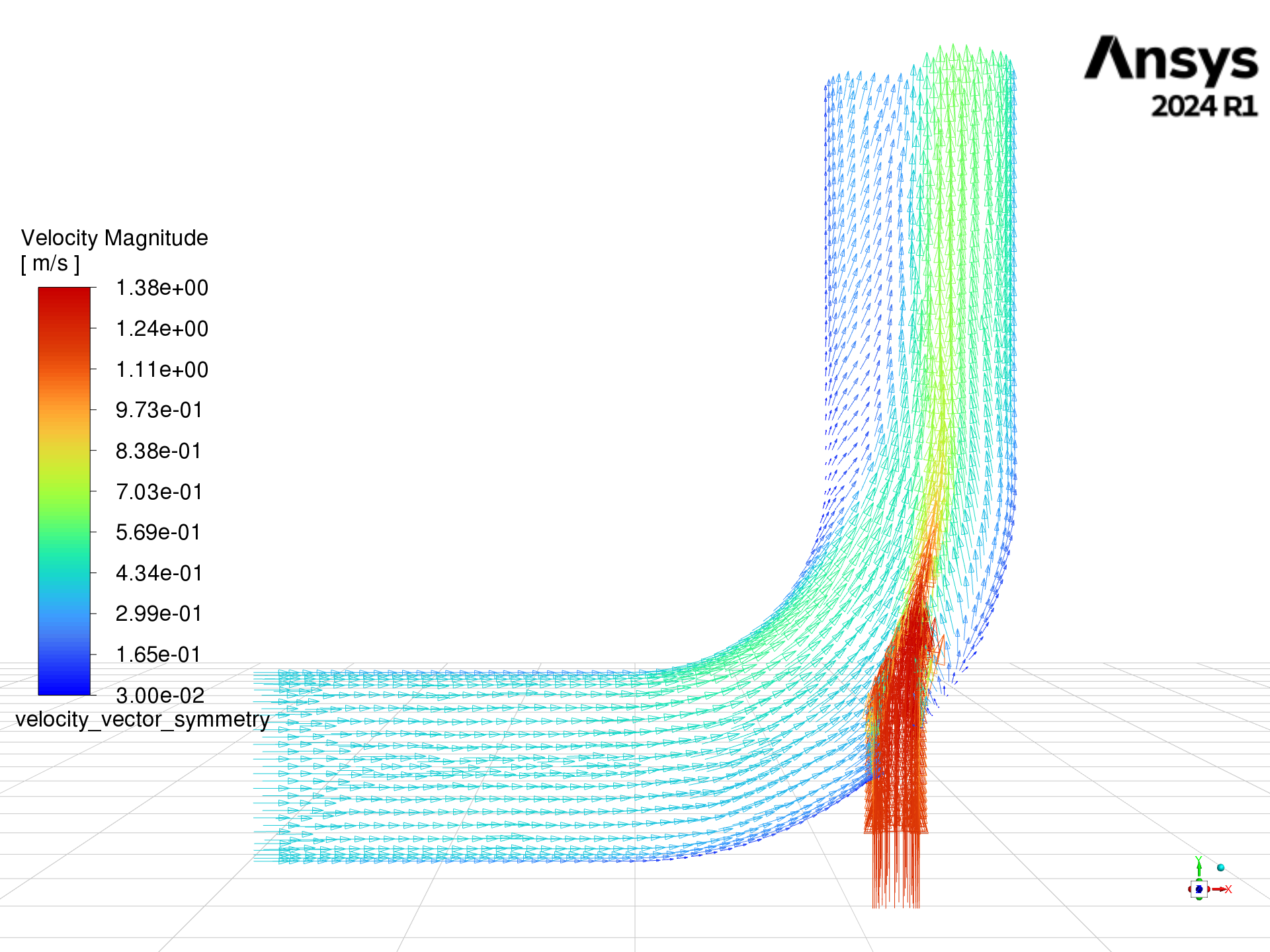
Create velocity vectors#
Create and display velocity vectors on the symmetry-xyplane plane, then
export the image for inspection.
graphics = solver_session.settings.results.graphics

graphics.vector["velocity_vector_symmetry"] = {}
velocity_symmetry = solver_session.settings.results.graphics.vector[
    "velocity_vector_symmetry"
]
velocity_symmetry.print_state()
velocity_symmetry.field = "velocity-magnitude"
velocity_symmetry.surfaces_list = [
    "symmetry-xyplane",
]
velocity_symmetry.options.scale = 4
velocity_symmetry.style = "arrow"
velocity_symmetry.display()

graphics.views.restore_view(view_name="front")
graphics.views.auto_scale()
graphics.picture.save_picture(file_name="velocity_vector_symmetry.png")
Compute mass flow rate#
Compute the mass flow rate.
solver_session.settings.solution.report_definitions.flux["mass_flow_rate"] = {}

mass_flow_rate = solver_session.settings.solution.report_definitions.flux[
    "mass_flow_rate"
]
mass_flow_rate.boundaries.allowed_values()
mass_flow_rate.boundaries = [
    "cold-inlet",
    "hot-inlet",
    "outlet",
]
mass_flow_rate.print_state()
solver_session.settings.solution.report_definitions.compute(
    report_defs=["mass_flow_rate"]
)
Close Fluent#
Close Fluent.
solver_session.exit()