Modeling Species Transport and Gaseous Combustion

Introduction

This tutorial examines the mixing of chemical species and the combustion of a gaseous fuel.

A cylindrical combustor burning methane (\(CH_4\)) in air is studied using the eddy-dissipation model in PyFluent.

This tutorial demonstrates how to do the following:

• Enable physical models, select material properties, and define boundary conditions for a turbulent flow with chemical species mixing and reaction.

• Initiate and solve the combustion simulation using the pressure-based solver.

• Examine the reacting flow results using graphics.

Problem Description

The cylindrical combustor considered in this tutorial is shown in the following figure. The flame considered is a turbulent diffusion flame. A small nozzle in the center of the combustor introduces methane at 80 m/s. Ambient air enters the combustor coaxially at 0.5 m/s. The overall equivalence ratio is approximately 0.76 (approximately 28% excess air). The high-speed methane jet initially expands with little interference from the outer wall, and entrains and mixes with the low-speed air. The Reynolds number based on the methane jet diameter is approximately \(5.7 × 10^3\).

Combustion of Methane Gas in a Turbulent Diffusion Flame Furnace

Background

In this tutorial, we will use the generalized eddy-dissipation model to analyze the methane-air combustion system. The combustion will be modeled using a global one-step reaction mechanism, assuming complete conversion of the fuel to \(CO_2\) and \(H_2O\). The reaction equation is

\[CH_4 + 2H_2O → CO_2 + 4H_2\]

This reaction will be defined in terms of stoichiometric coefficients, formation enthalpies, and parameters that control the reaction rate. The reaction rate will be determined assuming that turbulent mixing is the rate-limiting process, with the turbulence-chemistry interaction modeled using the eddy-dissipation model.

Setup and Solution

Preparation

Launch Fluent 2D in solution mode and print Fluent version.

import ansys.fluent.core as pyfluent

solver = pyfluent.launch_fluent(dimension=2)
print(solver.get_fluent_version())

Import some direct settings classes which will be used in the following sections. These classes allow straightforward access to various settings without the need to navigate through the settings hierarchy.

from pathlib import Path  # noqa: E402

from ansys.fluent.core import FluentVersion  # noqa: E402
from ansys.fluent.core.examples import download_file  # noqa: E402
from ansys.fluent.core.solver import (  # noqa: E402
    Contour,
    Energy,
    Mesh,
    MixtureMaterial,
    PressureOutlet,
    Species,
    Vector,
    VelocityInlet,
    Viscous,
    WallBoundary,
)

Mesh

Download the mesh file and read it into the Fluent session.

mesh_file = Path(
    download_file("gascomb.msh.gz", "pyfluent/tutorials/species_transport")
)
solver.settings.file.read_mesh(file_name=mesh_file)

General Settings

Check the mesh.

Fluent will perform various checks on the mesh and will report the progress in the console. Ensure that the reported minimum volume reported is a positive number.

solver.settings.mesh.check()

Scale the mesh and check it again.

Since this mesh was created in units of millimeters, we will need to scale the mesh into meters.

Note

We should check the mesh after we manipulate it (scale, convert to polyhedra, merge, separate, fuse, add zones, or smooth and swap). This will ensure that the quality of the mesh has not been compromised.

solver.settings.mesh.scale(x_scale=0.001, y_scale=0.001)
solver.settings.mesh.check()

Display the mesh in Fluent and save the image to a file to examine locally.

mesh = Mesh(solver, new_instance_name="mesh")
mesh.surfaces_list = mesh.surfaces_list.allowed_values()
mesh.display()
graphics = solver.settings.results.graphics
graphics.views.auto_scale()
if graphics.picture.use_window_resolution.is_active():
    graphics.picture.use_window_resolution = False
graphics.picture.x_resolution = 3840
graphics.picture.y_resolution = 2880
graphics.picture.save_picture(file_name="mesh.png")

The Quadrilateral Mesh for the Combustor Model

Inspect the available options for the two-dimensional space setting and set it to axisymmetric.

solver.settings.setup.general.solver.two_dim_space.allowed_values()

solver.settings.setup.general.solver.two_dim_space = "axisymmetric"

Models

Enable heat transfer by enabling the energy model.

Energy(solver).enabled = True

Inspect the default settings for the k-ω SST viscous model.

Viscous(solver).print_state()

Inspect the available options for the species model and set it to species transport.

species = Species(solver)
species.model.option.allowed_values()

species.model.option = "species-transport"

Inspect the species model settings.

species.print_state()

Enable volumetric reactions.

species.reactions.enable_volumetric_reactions = True

Set the material to methane-air.

Note

The available material list contains the set of chemical mixtures that exist in the Ansys Fluent database. We can select one of the predefined mixtures to access a complete description of the reacting system. The chemical species in the system and their physical and thermodynamic properties are defined by our selection of the mixture material. We can alter the mixture material selection or modify the mixture material properties using the material settings (see Materials).

species.model.material = "methane-air"

Set the turbulence-chemistry interaction model to eddy-dissipation.

The eddy-dissipation model computes the rate of reaction under the assumption that chemical kinetics are fast compared to the rate at which reactants are mixed by turbulent fluctuations (eddies).

species.turb_chem_interaction_model = "eddy-dissipation"

Inspect the species model settings after the changes.

species.print_state()

Materials

In this step, we will examine the default settings for the mixture material. This tutorial uses mixture properties copied from the Ansys Fluent database. In general, we can modify these or create our own mixture properties for our specific problem as necessary.

Print some specific properties of the mixture material (methane-air). We avoid printing the entire state of the mixture material to keep the output concise.

mixture_material = MixtureMaterial(solver, name="methane-air")
print(f"Species list: {mixture_material.species.volumetric_species.get_object_names()}")
print(f"Reactions option: {mixture_material.reactions.option()}")
print(f"Density option: {mixture_material.density.option()}")
print(f"Cp (specific heat) option: {mixture_material.specific_heat.option()}")
print(f"Thermal conductivity value: {mixture_material.thermal_conductivity.value()}")
print(f"Viscosity value: {mixture_material.viscosity.value()}")
if solver.get_fluent_version() < FluentVersion.v252:
    print(f"Mass diffusivity value: {mixture_material.mass_diffusivity.value()}")
else:
    print(
        f"Mass diffusivity value: {mixture_material.mass_diffusivity.constant_mass_diffusivity()}"
    )

Boundary Conditions

Convert the symmetry zone to the axis type.

The symmetry zone must be converted to an axis to prevent numerical difficulties where the radius reduces to zero.

solver.settings.setup.boundary_conditions.set_zone_type(
    zone_list=["symmetry-5"], new_type="axis"
)

Set the boundary conditions for the air inlet (velocity-inlet-8).

Set the zone name to air-inlet.

This name is more descriptive for the zone than velocity-inlet-8.

solver.settings.setup.boundary_conditions.velocity_inlet["velocity-inlet-8"].rename(
    "air-inlet"
)

Set the following boundary conditions for the air-inlet:

• Velocity magnitude: 0.5 m/s

• Turbulent intensity: 10%

• Hydraulic diameter: 0.44 m

• Temperature: 300 K

• Species mass fraction for o2: 0.23

air_inlet = VelocityInlet(solver, name="air-inlet")
air_inlet.momentum.velocity_magnitude = 0.5
air_inlet.turbulence.turbulence_specification = "Intensity and Hydraulic Diameter"
air_inlet.turbulence.turbulent_intensity = 0.1
air_inlet.turbulence.hydraulic_diameter = 0.44
air_inlet.thermal.temperature = 300
air_inlet.species.species_mass_fraction["o2"] = 0.23

Verify the state of the air-inlet boundary condition after the changes.

air_inlet.print_state()

Set the boundary conditions for the fuel inlet (velocity-inlet-6).

Set the zone name to fuel-inlet.

This name is more descriptive for the zone than velocity-inlet-6.

solver.settings.setup.boundary_conditions.velocity_inlet["velocity-inlet-6"].rename(
    "fuel-inlet"
)

Set the following boundary conditions for the fuel-inlet:

• Velocity magnitude: 80 m/s

• Turbulent intensity: 10%

• Hydraulic diameter: 0.01 m

• Temperature: 300 K

• Species mass fraction for ch4: 1

fuel_inlet = VelocityInlet(solver, name="fuel-inlet")
fuel_inlet.momentum.velocity_magnitude = 80
fuel_inlet.turbulence.turbulence_specification = "Intensity and Hydraulic Diameter"
fuel_inlet.turbulence.turbulent_intensity = 0.1
fuel_inlet.turbulence.hydraulic_diameter = 0.01
fuel_inlet.thermal.temperature = 300
fuel_inlet.species.species_mass_fraction["ch4"] = 1

Verify the state of the fuel-inlet boundary condition after the changes.

fuel_inlet.print_state()

Set the following boundary conditions for the exit boundary (pressure-outlet-9):

• Gauge pressure: 0 Pa

• Backflow turbulence intensity: 10%

• Backflow Hydraulic diameter: 0.45 m

• Backflow total temperature: 300 K

• Backflow species mass fraction for o2: 0.23

The Backflow values in the pressure outlet boundary condition are utilized only when backflow occurs at the pressure outlet. Always assign reasonable values because backflow may occur during intermediate iterations and could affect the solution stability.

pressure_outlet = PressureOutlet(solver, name="pressure-outlet-9")
pressure_outlet.momentum.gauge_pressure = 0
pressure_outlet.turbulence.turbulence_specification = "Intensity and Hydraulic Diameter"
pressure_outlet.turbulence.backflow_turbulent_intensity = 0.1
pressure_outlet.turbulence.backflow_hydraulic_diameter = 0.45
pressure_outlet.thermal.backflow_total_temperature = 300
pressure_outlet.species.backflow_species_mass_fraction["o2"] = 0.23

Verify the state of the pressure-outlet boundary condition after the changes.

pressure_outlet.print_state()

Set the boundary conditions for the outer wall (wall-7).

Set the zone name to outer-wall.

This name is more descriptive for the zone than wall-7.

solver.settings.setup.boundary_conditions.wall["wall-7"].rename("outer-wall")

Set the following boundary conditions for the outer-wall:

• Temperature: 300 K

outer_wall = WallBoundary(solver, name="outer-wall")
outer_wall.thermal.thermal_condition = "Temperature"
outer_wall.thermal.temperature = 300

Verify the state of thermal properties of the outer-wall boundary condition after the changes.

outer_wall.thermal.print_state()

Set the boundary conditions for the fuel inlet nozzle (wall-2).

Set the zone name to nozzle.

This name is more descriptive for the zone than wall-2.

solver.settings.setup.boundary_conditions.wall["wall-2"].rename("nozzle")

Set the following boundary conditions for the nozzle for adiabatic wall conditions:

• Heat flux: 0 \(W/m^2\)

nozzle = WallBoundary(solver, name="nozzle")
nozzle.thermal.thermal_condition = "Heat Flux"
nozzle.thermal.heat_flux = 0

Verify the state of thermal properties of the nozzle boundary condition after the changes.

nozzle.thermal.print_state()

Reaction Solution

We will calculate a solution for the reacting flow.

Inspect the solution methods settings.

solver.settings.solution.methods.print_state()

Ensure that plot is enabled in residual monitor options.

solver.settings.solution.monitor.residual.options.plot()

Initialize the field variables.

solver.settings.solution.initialization.hybrid_initialize()

Save the case file (gascomb1.cas.h5).

solver.settings.file.write_case(file_name="gascomb1.cas.h5")

Run the calculation for 200 iterations.

solver.settings.solution.run_calculation.iterate(iter_count=200)

Set time scale factor to 5.

The Time Scale Factor allows us to further manipulate the computed time step size calculated by Fluent. Larger time steps can lead to faster convergence. However, if the time step is too large it can lead to solution instability.

solver.settings.solution.run_calculation.pseudo_time_settings.time_step_method.time_step_size_scale_factor = (
    5
)

Run the calculation for 200 iterations.

solver.settings.solution.run_calculation.iterate(iter_count=200)

Save the case and data files (gascomb1.cas.h5 and gascomb1.dat.h5).

solver.settings.file.write_case_data(file_name="gascomb1.cas.h5")

Postprocessing

Review the solution by examining graphical displays of the results and performing surface integrations at the combustor exit.

Report the total sensible heat flux. We shall use wildcards to specify all zones.

solver.settings.results.report.fluxes.get_heat_transfer_sensible(zones="*")

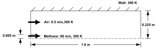
Display filled contours of temperature and save the image to a file.

contour1 = Contour(solver, new_instance_name="contour-temp")
contour1.field = "temperature"
contour1.surfaces_list = contour1.surfaces_list.allowed_values()
contour1.coloring.option = "banded"
contour1.display()
graphics.views.auto_scale()
# graphics.picture.save_picture(file_name="contour-temp.png")

Contours of Temperature

The peak temperature is approximately 2300 K.

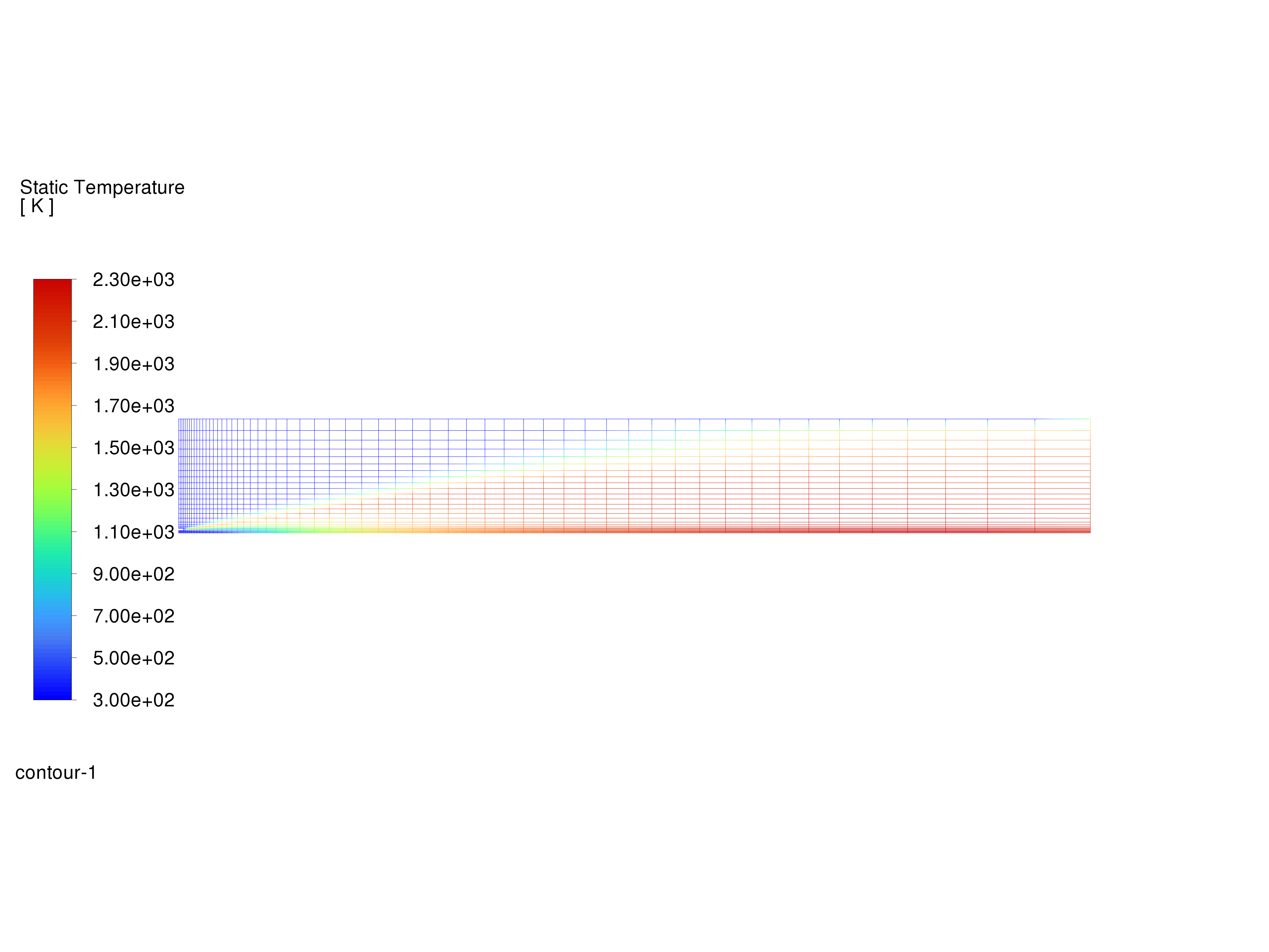
Display velocity vectors and save the image to a file.

vector1 = Vector(solver, new_instance_name="vector-vel")
vector1.surfaces_list = ["interior-4"]
vector1.scale.scale_f = 0.01
vector1.vector_opt.fixed_length = True

The fixed length option is useful when the vector magnitude varies dramatically. With fixed length vectors, the velocity magnitude is described only by color instead of by both vector length and color.

vector1.vector_opt.scale_head = 0.1
vector1.display()
graphics.views.auto_scale()
graphics.picture.save_picture(file_name="vector-vel.png")

Velocity Vectors

The entrainment of air into the high-velocity methane jet is clearly visible.

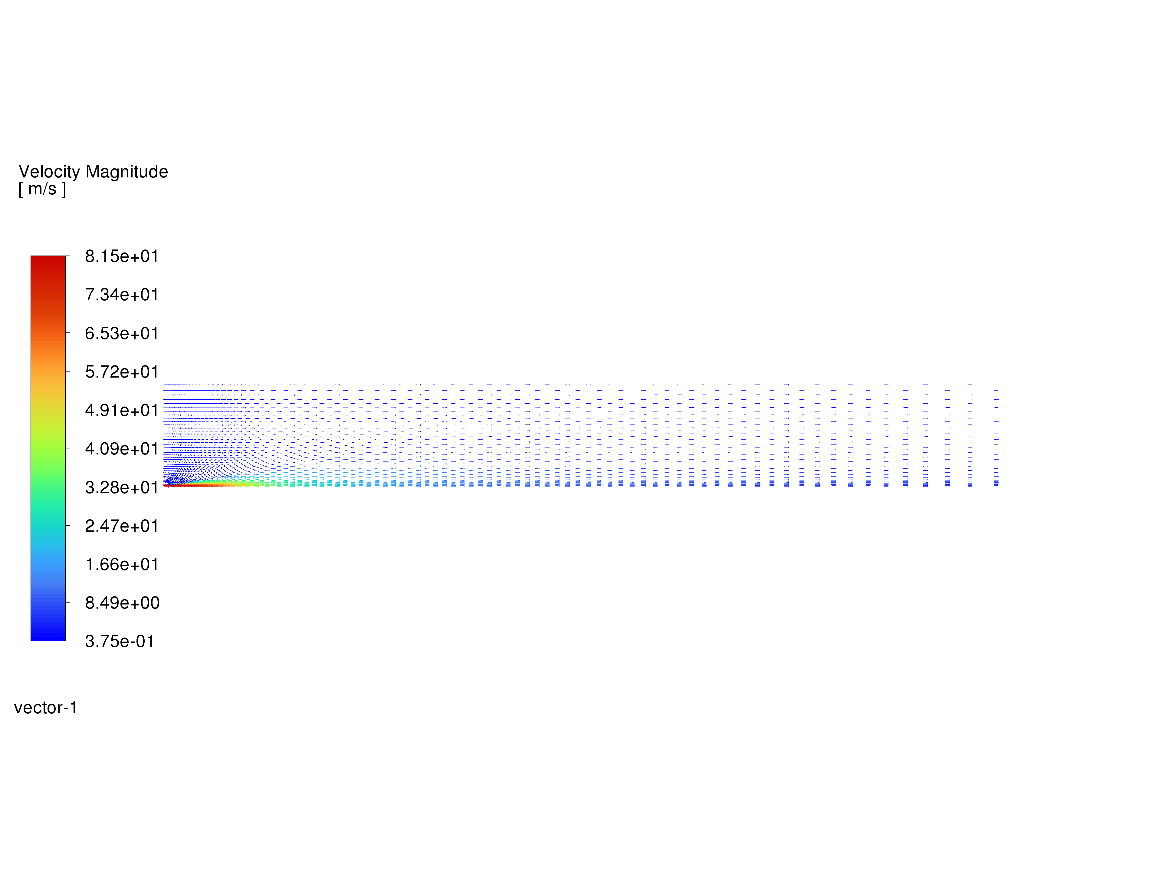
Display filled contours of mass fraction of \(CH_4\) and save the image to a file.

contour2 = Contour(solver, new_instance_name="contour-ch4-mass-fraction")
contour2.field = "ch4"
contour2.surfaces_list = contour2.surfaces_list.allowed_values()
contour2.display()
graphics.views.auto_scale()
graphics.picture.save_picture(file_name="contour-ch4-mass-fraction.png")

Contours of \(CH_4\) Mass Fraction

Display filled contours of mass fraction of \(O_2\) and save the image to a file.

contour3 = Contour(solver, new_instance_name="contour-o2-mass-fraction")
contour3.field = "o2"
contour3.surfaces_list = contour3.surfaces_list.allowed_values()
contour3.display()
graphics.views.auto_scale()
graphics.picture.save_picture(file_name="contour-o2-mass-fraction.png")

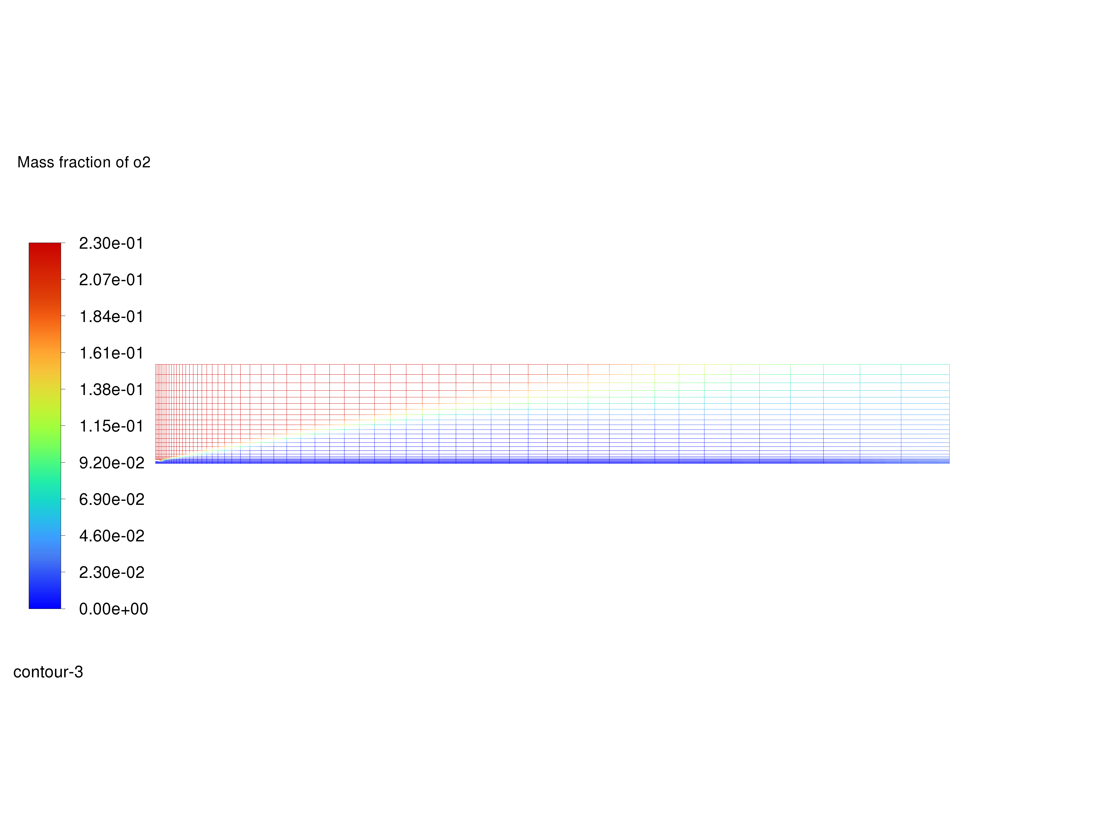
Contours of \(O_2\) Mass Fraction

Display filled contours of mass fraction of \(CO_2\) and save the image to a file.

contour4 = Contour(solver, new_instance_name="contour-co2-mass-fraction")
contour4.field = "co2"
contour4.surfaces_list = contour4.surfaces_list.allowed_values()
contour4.display()
graphics.views.auto_scale()
graphics.picture.save_picture(file_name="contour-co2-mass-fraction.png")

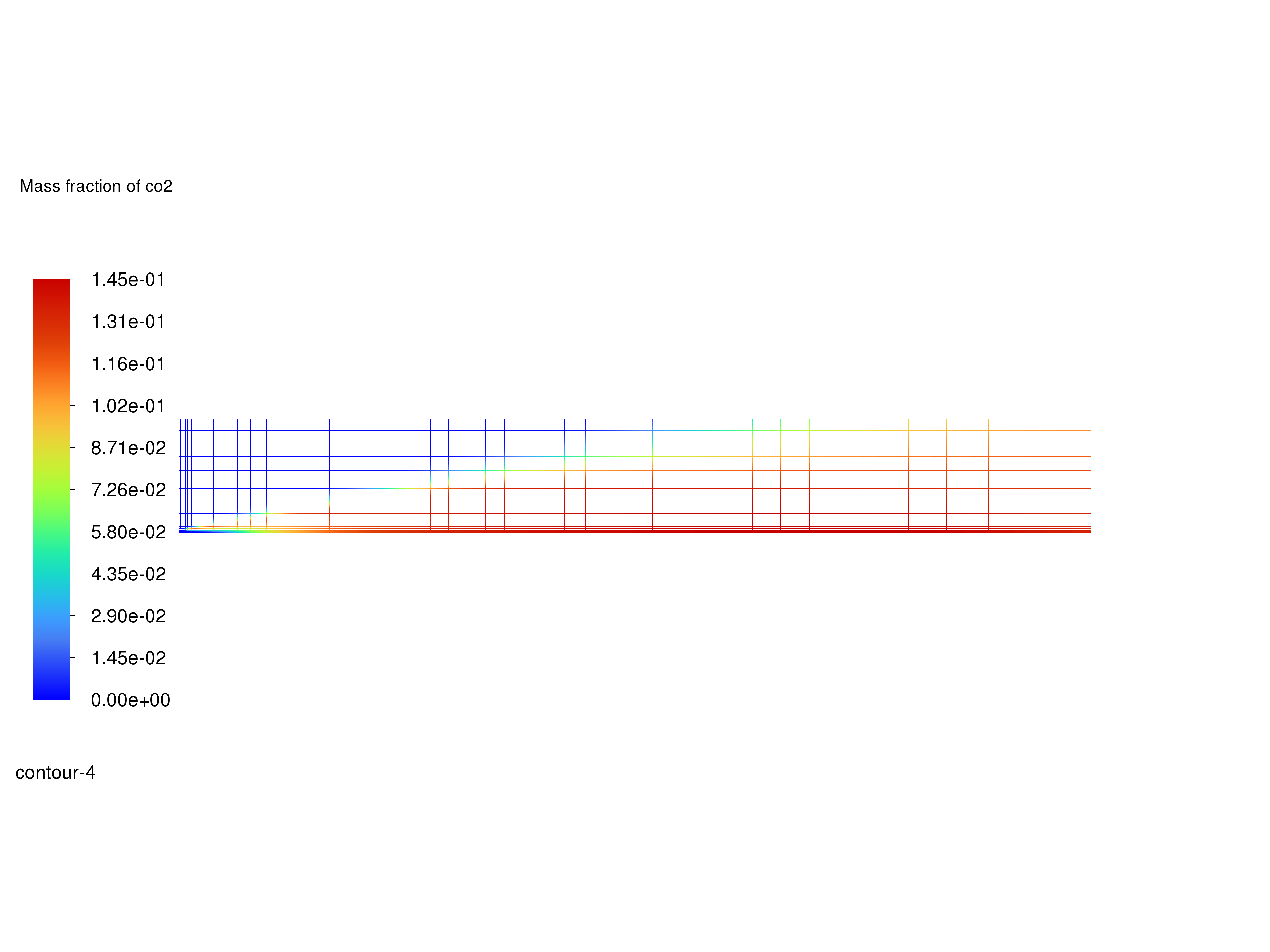
Contours of \(CO_2\) Mass Fraction

Display filled contours of mass fraction of \(H_2O\) and save the image to a file.

contour5 = Contour(solver, new_instance_name="contour-h2o-mass-fraction")
contour5.field = "h2o"
contour5.surfaces_list = contour5.surfaces_list.allowed_values()
contour5.display()
graphics.views.auto_scale()
graphics.picture.save_picture(file_name="contour-h2o-mass-fraction.png")

Contours of \(H_2O\) Mass Fraction

Determine the average exit temperature.

The mass-averaged temperature will be computed as:

\[\bar{T}=\frac{\int T \rho \vec{v} \cdot d \vec{A}}{\int \rho \vec{v} \cdot d \vec{A}}\]

The mass-averaged temperature at the exit is approximately 1840 K.

solver.settings.results.report.surface_integrals.get_mass_weighted_avg(
    report_of="temperature", surface_names=["pressure-outlet-9"]
)

Determine the average exit velocity.

The mass-averaged velocity will be computed as:

\[v=\frac{1}{A} \int v d A\]

The Area-Weighted Average field will show that the exit velocity is approximately 3.37 m/s.

solver.settings.results.report.surface_integrals.get_area_weighted_avg(
    report_of="velocity-magnitude", surface_names=["pressure-outlet-9"]
)

Save the case file (gascomb1.cas.h5).

solver.settings.file.write_case(file_name="gascomb1.cas.h5")

Close Fluent

solver.exit()

Summary

In this tutorial we used PyFluent to model the transport, mixing, and reaction of chemical species. The reaction system was defined by using a mixture-material entry in the Ansys Fluent database. The procedures used here for simulation of hydrocarbon combustion can be applied to other reacting flow systems.